Matteo Capuccihttps://matteocapucci.eu/matteo-capucci/2026-03-05https://matteocapucci.eu/feed/https://matteocapucci.eu/feed/Quanta Article on Applied Category Theory2026-03-05T00:00:00Z2026-03-05T00:00:00ZMatteo Capuccihttps://matteocapucci.eu/matteo-capucci/https://matteocapucci.eu/quanta-article/
Natalie Wolchover wrote a column on Quanta magazine about applied category theory, mainly centering around John Baez but also interviewing many other people from the community, including yours truly!
This is the first time I'm interviewed in my capacity as a mathematician.
It was really fun to articulate to Natalie what applied category theory is, and what it is good for.
She got this quote out of me:
When I say we’re underdogs and nobody likes us, it’s not completely true, but it’s a bit true.
which sounds a bit self-aggrandizing, but didn't want to be.
Applied category theory is a bit niche, sometimes dismissed as needlessly abstract and naive, but mostly respected.
How to deploy a Forest to GitHub Pages2026-02-17T00:00:00Z2026-02-17T00:00:00ZMatteo Capuccihttps://matteocapucci.eu/matteo-capucci/https://matteocapucci.eu/how-to-deploy-forester-to-github-pages/
So you have grown a beautiful Forester forest on your machine. It is structured, it is evergreen, and the mathematical diagrams render perfectly. Naturally, you want to share it with the world via GitHub Pages. Despite it being quite easy in the end, I spent a lovely afternoon untangling 404 errors, mysterious XSLT parsing failures, and OCaml version mismatches. So here is a short guide to share what I learned in the process, for when I will inevitably forget everything.
The website is deployed by a GitHub Actions workflow that installs a minimal TeX Live (for those sweet diagrams), set up OCaml 5.3+ (required for Forester 5.0), installs forester, builds the forest, and ship it to Pages.
I used the zauguin/install-texlive action for TeX to keep things lightweight, and the standard ocaml/setup-ocaml with caching enabled. You can see my full workflow file here: .github/workflows/forester.yml.
Installing the full TeX Live distribution on CI is a massive waste of bandwidth and time. The good thing about zauguin/install-texlive is that you can easily instruct it to pull down a minimal installation.
The package list was built by grepping around the repo for package names, and scheme-basic takes care of most of the essentials. Also keep in mind a package name in LaTeX is not necessarily the package name tlmgr expects—gotta confess that Gemini was really helpful in figuring out this one.
The first real pitfall I encountered was that the latest Forester (5.0+) strictly requires OCaml 5.3 or newer. If you just ask for ocaml-compiler: 5.x, you might get 5.2, which causes Opam to quietly fall back to Forester 4.3.1. Suddenly your new features vanish and you are debugging ghost bugs.
Thus we have to pin the version we need:
- name: Setup OCaml
        uses: ocaml/setup-ocaml@v3
        with:
          # Forester 5.0 requires OCaml >= 5.3.0
          ocaml-compiler: 5.3
          dune-cache: true

      - name: Install Forester
        # Pinning the version ensures we get 5.0 or fail if incompatible
        run: opam install forester.5.0
Finally, remember to add this block to give the action permission to deploy.
The last hurdle I had to jump was a bit of delicate configuration regarding base URLs. A good piece of debugging advice is that if you end up with a site that loads but throws "XSLT parsing errors" there is a good chance your XSLTs are 404ing, and the culprit is likely how Forester calculates base URLs when deploying to a project subdirectory. Then using browser networking tools you can see which XSL files the browser is trying to load.
All in all, keep in mind Forester is sensitive to the url setting in forest.toml and its trailing slashes. If you look at my configuration in forest.toml, you will see this:
[forest]
trees = ["trees"]
assets = ["assets"]
url = "https://mattecapu.github.io/website/"
home = "matteo-capucci/"
It's important the slashes are where they are.
Because I set the URL to include /website/, Forester infers that the base path is /website/. Consequently, it builds everything into an ulterior subfolder named after that path inside the output directory.
In practice, this means that in the workflow we simply account for that:
Thanks to Eigil Fjeldgren Rischel for catching a mistake in an earlier version of this post (see comment below).
Let \cal K be a monoidal closed 2-category with left Kan extensions and let T:\cal K \to \cal K be a lax monoidal endofunctor over it. Suppose V and A are T-algebras.
Often we want to define T-convolution of ‘functions’ A \to V, an operation that carries ‘T-terms’ of functions A\to V into new functions A \to V. In other words, a T-algebra structure on [A, V].
The paradigmatic example here is Day convolution, where \cal K= \bf Cat, V = \bf Set and T is the free monoidal category 2-monad. There, a ‘T-term of functions’ is a tuple of copresheaves A \to \bf Set over a monoidal category A. Day convolution gives you a new copresheaf on A from this data.
Another example is ‘Day convolaction’, which I previously described in Tambara modules are modules. In that case we have \cal K=\bf Cat and V=\bf Set again but T is the free \cal M-actegory 2-monad. Then Day convolaction endows [A,V] with an \cal M-action. (In fact it endows it with a whole [\cal M, V]-action, showing the following can be generalized further by replacing monads with graded monads, though, notably, Tambara theory only use the \cal M-action!).
The description of T-convolution is really simple. It’s made of three pieces:
T is a lax monoidal functor, thus in particular lax closed, meaning there are coherent maps:
T[A,V] \to [TA, TV]
V is a T-algebra, thus induces a map by post-composition:
[TA,TV] \to [TA, V]
Finally, \cal K is closed so the T-algebra structure on A induces a map by left Kan extension:
[TA,V] \to [A,V]
Composing these maps gives you the desired T-algebra structure on [A,V].
An observation is: one could replace left Kan extension with any contravariant aggregation operation. This is especially useful when decategorifying the above, in which case one might replace the colimits involved in a Kan extension with e.g. sums in V. See pull-tensor-push.
Warning: the following is a bit speculative.
The above should work for {\cal K}={\bf Cat}/O, where O is a category of interfaces, and T is the 2-monad associated to a double operad\cal W of wiring operations with colours O. Now a T-algebra is a theory of systems indexed by \cal W. Let V be some other algebra, usually it’s something involving sets indexed by colours.
Then we can talk about \cal W-convolution of ‘quantities’ A \to V: given quantities (q_i:A(o_i) \to V(o_i))_{o_1, \ldots , o_n} and an operation w:o_1, \ldots , o_n \to o in \cal W, we can convolve the first along w to obtain w \ast (q_1, \ldots , q_n) : A(o)\to V(o).
Note that, crucially, we need \cal W to be double to be able to perform a Kan extension. In other words, we need to know how systems map into each other to know how to aggregate quantities on them.
I don’t know yet what I want to do with this operation but I suspect it might be useful to study compositionality of quantities defined over systems, chiefly behaviours.
A glimpse of the algebraic theory of linear systems2024-03-01T00:00:00Z2024-03-01T00:00:00ZMatteo Capuccihttps://matteocapucci.eu/matteo-capucci/https://matteocapucci.eu/a-glimpse-of-the-algebraic-theory-of-linear-systems/
I’ve been in Berkeley for the last two weeks, having lots of mathematical fun at Topos in the context of a workshop on Poly.
I focused on its links with categorical systems theory, chatting with lots of people about it. With Sophie Libkind and Toby St Clere Smithe we found a bridge between the theory of dynamic operads of David Spivak and Brandon Shapiro, the animated categories of Toby, and the cybernetic systems theories of mine. I also managed to make Sophie not scared but actually delighted by categorical systems theory, the way it handles behaviour, and the beauty of it all. Yu-uh!
But here I’d like to report about some of the amazing things I’ve learned from Mohamed Barakat. He’s a computational algebraist, i.e. someone who makes computers do algebra for us (yay!), who’s recently been applying the methods of his discipline to the theory of linear systems. It turns out Kalman’s dream of reducing linear systems theory to homological algebra is alive and well, and it’s now broadly developed in algebraic systems theory.
In algebraic systems theory, one starts from an algebra of operatorsD. These can be differential operators (partial or not!), difference operators, time-shift operators and more (this theory is very general!). One then uses operators from D to write down the equations of a system. For instance we might take D to be the Weyl algebra of differential operators on \mathbb {R}^3 and write equations
\begin {cases} 3\partial _t x - u = 0\\ (\partial _t)^2 x = \partial _x^2 x\\ y = x\\ z = u\\ \end {cases}
This is a linear system of 2 equations in the 4 variables x,y,z,u with coefficients in D, which in this (and most) case(s) is a kind of polynomial algebra. Notice that the variables are all treated equally, but display some attitude: x looks a like a state variable, u like a control one, and y,z like observables.
We now hit this with lots of interesting homological algebra, i.e. linear algebra on steroids. The starting point is to present our equations as a matrix multiplication:
Denote by E for the big matrix of operators. We can see it as a morphism of D-modules E : D^4 \to D^4, whose cokernel represents the equations themselves as a further D-module:
D^4 \xrightarrow {E} D^2 \twoheadrightarrow \operatorname {coker} E
In this way, morphisms from \operatorname {coker} E to any other D-module M, such as {\cal C}^\infty (\mathbb {R}^n) corresponds to solutions of E in M.
In fact now one can ‘kick the ladder’ and think of any finitely-presented D-module S as a linear system. Now we can formulate properties of the systemS as homological properties of the moduleS translate to properties of the system described by S.
As an example, Mohamed showed me the following application, which I hope I’m not going to butcher. One can compute a spectral sequence related to the derived functor \operatorname {Hom}(\operatorname {Hom}(-, D), D) (take the double dual of a resolution of S) and find a presentation of S as a matrix algebra (he called it an equidimensional decomposition):
where each block S_i represents the ‘autonomy of degree i’ of S, where the latter roughly means individuation a subsystem of S which is governed by i-many ‘conservation laws’ which prevent control. Algebraically, these are degrees of torsion, since a conservation law is nothing but an operator d \in D such that ds=0 for some element s \in S.
S_0 is the part that doesn’t respect any conservation law, but still might not be controllable: there might be other kinds of constraints, or simply couplings, expressed by equations such as ds + d's' = 0, which even though don’t give rise to an autonomous subsystem of S, constrain its controllability. One can in fact compute a further decomposition of S_0 into more and more controllable parts.
A dual theory concerns observability instead, and allows one to decompose S into various degree of observability!
Moreover, Mohamed didn’t just tell me about this. He is a computational algebraist after all, so he has the means to actually compute the above homological construction, and indeed he showed me a live demo on Maple on how to solve exactly a complicated PDE in mere seconds by purely homological methods. I’m still astounded!
If you are as avid of reading more as me, Mohamed suggested to consult his webpage (linked above). Also, this paper of his student Sebastian Posur paints a better picture than I did above of this wonderful theory.
Meeting Mohamed what such a great pleasure. He blew my mind with incredible math, and he refreshed me with an uncommon balanced attitude for someone working at the interface of theory and applications, never disowning either side. And he taught me why spectral sequences work!
I look forward working with him in the future, perhaps extending the algebraic theory of linear systems with compositionality results.
Induction is induction2024-02-23T00:00:00Z2024-02-23T00:00:00ZMatteo Capuccihttps://matteocapucci.eu/matteo-capucci/https://matteocapucci.eu/induction-is-induction/
David Corfield made a very interesting observation: the three types of logical reasoning of Peirce’s, deduction, induction, abduction, correspond to three very elementary operations in category theory: composition, extension and lifting.
Let’s see what this means.
Deduction. I observe A \to B and B \to C. Then, by modus ponens, I can conclude A \to C.
Induction. I observe A \to B, and also A \to C. I conclude B \to C.
Abduction. I observe A \to C and B \to C, I conclude A \to B.
Clearly induction and abduction are not valid reasoning rules! But they are rules reasoners have to use if they want to make new knowledge out of the data they have. For instance, we use induction all the time, both ‘unconsciously’ when we learn facts from the world (‘I said the word mama, mama smiled, therefore the word mama makes mama smile’) and very consciously in science (‘We collected these data samples, and we infer a functional relationship of this kind’).
In fact you can see how the data for induction is literally the data of an indexed family of pairs (a_i, b_i)_{i \in I}, and the result of induction is to build a map f:A \to B such that f(a_i) = b_i for each i \in I: it’s an interpolation problem!
But, again, this isn’t a valid logical rule: there might not be such f, since e.g. there might a_i=a_j with b_i \neq b_j (so no function can interpolate the points), or even if the points are possible to interpolate, there’s just so many different functions that do so!
So to give some logical credence to induction, we have to find a way to at least solve the second problem, and thus make induction the more conservative conclusion we can make having observed that I \to A and I \to B. In other words, solve the extension problem in a universal way.
This is the job for a Kan extension!
This means, first of all, moving from the unspecified 1-category I’ve been working on so far to an unspecified 2-category. Then a (right) Kan extension looks as follows:
The dashed arrow and the filling 2-cell are terminal at their job: every other such pair factors uniquely through them:
So this is the sense in which {\rm ran}_a b is the ‘least general solution’ to this extension problem: every other solution factors through it. The right Kan extension only contains what’s justified to believe about the implication A \to B.
There is also a nice formula for computing {\rm ran}_a b in reasonable cases, if it exists:
{\rm ran}_a b(a) = {\large \textstyle \int _{i:I} \int _{p:A(a,a_i)} b_i}
An interpretation of this formula is that the value of the interpolation of (a_i,b_i)_i at some given point a is the limit over i of all the values b_i which lie over an a_i related to a. In other words, we ‘fill the gaps’ in the data by taking limits.
Of course this is far from what actual interpolation looks like, a problem which requires spending a bit more time thinking about what are the right generalizations for all these concepts to a ‘quantitative’ setting.
Still, we can test the proposed definition of ‘induction’ on something else: Peano induction! Is it a special case of induction? I claim it is.
What is mathematical induction? We are given a predicate \varphi : \mathbb {N}_0 \to 2, where \mathbb {N}_0 is the set of natural numbers, which we know satisfy \varphi (k) \to \varphi (k+1) and \varphi (b) for some b \in \mathbb {N}. We conclude that \forall n \in \mathbb {N},\ (b \leq n) \to \varphi (n).
So let’s work in \bf Pos, the 2-category of posets. We have a map i:\mathbb {N}_0 \to \mathbb {N} embedding the set of naturals in the poset of naturals. We have a predicate on \mathbb {N}_0. We form its right Kan extension:
Such a Kan extension has form
{\rm ran}_i \varphi (k) = \forall {n \in \mathbb {N}},\ (k \leq n) \to \varphi (n)
which reads as ‘{\rm ran}_i \varphi (k) is true when \varphi is always true from k onwards’.
How is this any useful for induction? Well, when \varphi satisfy the induction property then \varphi :\mathbb {N}_0 \to 2 actually lifts to \mathbb {N} \to 2, since \varphi (k) \to \varphi (k+1) is a monotonicity property.
Then by universal property of the Kan extension, there is a (necessarily unique in this context) map into it:
This map corresponds to the implication
\forall k \in \mathbb {N},\ \varphi (k) \to \forall {n_0 \in \mathbb {N}_0}\ (k \leq n_0) \to \varphi (n_0)
which is equivalent to
\forall k \in \mathbb {N}, \forall n \in \mathbb {N}, \varphi (k) \land (k \leq n) \to \varphi (n).
Then given a base case \varphi (b)=\top , we can conclude
\forall n \in \mathbb {N}, (b \leq n) \to \varphi (n).
So induction is a form of... induction after all!
What I really proved above is that for any poset W, right extension along the inclusion i:W_0 \to W gives you well-founded induction. Indeed, for general posets we have
{\rm ran}_i\varphi (v) = \forall w \in W, (v \leq w) \to \varphi (w)
and ‘functoriality’ of \varphi is
v \leq w \implies \varphi (v) \to \varphi (w)
Thus the universal map \varphi \to {\rm ran}_i\varphi says that
\forall v \in W,\ \varphi (v) \to (\forall w \in W, (v \leq w) \to \varphi (w))
which is easily seen to be equivalent to
\forall w \in W,\ (\forall v\in W, (v \leq w) \to \varphi (v)) \to \varphi (w).
Of course this extends to categories as well, where you’d get some kind of ‘proof-relevant’ induction. One can give the same definition anywhere you can talk about right Kan extensions and the inclusion W_0 \to W.
In my latest post on Tambara modules, I’ve shown you that if \mathcal C, \mathcal D are \mathcal M-actegories then the free Tambara module construction \Psi : \bf Prof(\mathcal C, \mathcal D) \to Tamb(\mathcal C, \mathcal D) is basically the free \mathcal M-action construction, where \mathcal M denotes the hom profunctor on \mathcal M and ‘action’ means ‘Day convolaction’.
Recall Day convolaction extends an \mathcal A-actegory structure on \mathcal X to an [\mathcal A^{op}, \bf Set]-actegory structure on [\mathcal X^{op}, \bf Set]. One can use this actegory structure as a way for monoids in [\mathcal A^{op}, \bf Set] to act on objects of [\mathcal X^{op}, \bf Set]. Above, I’m talking about this instanced for \mathcal A = \mathcal M \times \mathcal M^{op} and \cal X = C \times D^{op}—thus getting an action of \bf Prof(\cal M,M) on \bf Prof(\cal C,D)—and then looking at actions of the monoid \mathcal M(-,=): \cal M \nrightarrow M.
It was shown by Pastro and Street, but also by Mario Romàn and others, that \Psi \dashv U \dashv \Theta , where U is the forgetful functor from Tambara modules to profunctors, and \Theta is the functor:
\Theta P(C,D) = \int _M P(MC, MD).
In fact, this functor is the first one usually introduces when starting Pastro-Street theory of Tambara modules, since it’s very easy to see that coalgebras of \Theta U are strengths.
Indeed, a strength is a natural family \mathsf {st}_M^{C,D}:P(C,D) \to P(MC,MD) and these maps are classified by the end above by definition!
Once we established Tambara modules are actions of \mathcal M, and that \Psi \dashv U is monadic, then \Theta has to be the cofree action construction! I’ve been overlooking this fact since I didn’t know that Day convolaction is always left-closed, meaning acting by P-:\bf Prof(\cal C,D) \to \bf Prof(\cal C,D) has parametric right adjoint -/P:\bf Prof(\cal C,D) \to \bf Prof(\cal C,D) (this is different from right-closed, where it’s receiving an action which has a right adjoint, see Janelidze-Kelly).
I’ll give a definition for profunctors straight away, but of course this works for general presheaves:
For P:\cal M \nrightarrow M monoidal profunctor and Q:\cal C \nrightarrow D, define Q/P:\cal C \nrightarrow D as
Q/P(C,D) = \int _{MM'} \int _{C'D'} \mathcal C(C', MC) \times P(M,M') \times \mathcal D(M'D, D') \to Q(C',D').
Then it’s easy to see that -/\cal M \cong \Theta , by using a couple of Yoneda reductions:
Q/{\cal M}(C,D) = \int _{MM'} \int _{C'D'} \mathcal C(C', MC) \times {\cal M}(M,M') \times \mathcal D(M'D, D') \to Q(C',D')\\ \cong \int _{M} \int _{C'D'} \mathcal C(C', MC) \times \mathcal D(MD, D') \to Q(C',D')\\ \cong \int _{M} Q(MC,MD) = \Theta Q(C,D).
Argmax is my nemesis. It keeps popping up everywhere in my work and yet escapes a structuralist treatment. It has very bad formal properties and thus it’s hard to justify (which means saying argmax is ‘just’ a blah in a blah). That makes me mad!
For now, let’s work in \bf Cat. Consider a functor f:X \to V therein (typicially, f:X \to \mathbb {R} where X is discrete). An object x^* \in X is in the argmax iff fx^* is “terminal in the image of f”, i.e. iff for all x \in X, there exists a (perhaps unique) fx \to fx^*.
If one tries to read this as a universal property they are going to get all dizzy. The universal quantification ranges over objects of X but the invoked comparison maps are in V. This is weird.
One can frame \argmax as follows: consider the map f:X \to \mathbb {R} as a map of sets, and use it to pullback the order structure on \mathbb {R} onto X. This makes X look like the ‘level sets’ of f since x \leq x' \iff fx \leq fx', and thus in particular x \cong x' \iff fx = fx'. Then \argmax f is the isomorphism class of terminal objects in X.
‘Pulling back’ the order structure can be seen in various way. One is as a literal cartesian lift for the forgetful functor U:\bf Ord \to Set from orders to sets, which turns out to be a fibration. Indeed, the level sets construction is literally the functor \mathsf {lvl} : {\bf Set}/ U \to \bf Ord defining a cleavage for this fibration. Moreover {\bf Set}/U has a neat interpretation as ‘sets with utility’, and thus \mathsf {lvl} is a case of very natural and concrete construction (sending a utility function to its induced preference relation) having a decent universal property (being a right adjoint, being a cartesian lift functor, etc.).
That’s already quite cool! Let’s make this cooler by summoning equipments.
The operation of taking level sets can also be seen as follows: given a functor f:X \to V, one factors it as X \to \mathsf {lvl}f \to V where the first is a bijective-on-objects functor and the second is a fully-faithful functor (think: bijective-on-morphisms functor). Formally, this factorization comes from the a vertical-cartesian factorization system on \bf Cat induced by its fibration of objects \rm Ob: \bf Cat \to Set, which in turn is just an extension to categories of the fibration U above.
One can see this factorization in yet another way, by approaching categories as monads in spans. Recall that functors are tight maps in that equipment, thus in particular squares
where X_0,V_0 are the set of objects of X and V respectively, X_1 and V_1 the spans of morphisms, and f_0 and f_1 are similarly the action of f on objects and maps.
Now by being an equipment, we know this square has to factor along a restriction, thus yielding:
and this is basically the bo/ff factorization of f we had above. In fact it’s exactly the same since the 2-cell I labeled \text {cart} is the cartesian lift of the ‘category structure’ on V along the map of objects f_0.
But we can do something a bit different now. Let’s switch to think about this in the equipment \bf \mathbb Cat = \mathbb Mod(\mathbb Set) of categories, functors, profunctors and transformations. There, we can restrict the identity profunctor on V = (V_0, V_1) along the entire functor f, yielding:
Now V(f,f) is extra structure on the category X: it’s a promonad on it, thus the data of new morphisms on X, namely the ones it would have ‘in V’. This seems useful to talk about properties of elements of X with respect to morphisms between their f-images!
Besides, here’s a crucial insight: \argmax f should really be thought as a predicate on X. For instance, consider things like \mathrm {softmax} which assign a ‘maximality score’ to all things in a set: this smells a lot like literally argmax but seen as a ‘generalized predicate’ X \to [0,1]. And even without resorting to generalization, in a constructive setting one ends up encoding \argmax f as the X-indexed type which assign to each x the type of proofs of its argmaximality, in a classic proposition-as-types move.
So here’s a conjecture (I’m sure duality is gonna bite me): take the following lift in \bf Prof, the bicategory (you could probably swap if for the equipment above but I just don’t know how would that work):
By duality, one can compute this as a Kan extension, specifically (I’m stealing this idea from the nLab):
\argmax f = \mathsf {Rift}_1V(x^*) = \int _{x:X} (1(x) \to V(fx,fx^*)) = \int _x V(fx, fx^*)
where we are considering profunctors 1 \nrightarrow X directly as copresheaves over X.
It’s not hard to convince oneself that the above formula corresponds to defining:
x^* \in \argmax f \iff \forall x\in X,\ fx \leq fx^*.
Clearly, had we setup the above in the 2-\bf \mathbb Prof (aka \bf \mathbb Mod(\mathbb Rel)), this is exactly what we would have found!
Moreover, in this fashion, we can also describe constrained optimization problems. Say you have P:X \to \bf 2 \hookrightarrow Set describing the predicate which constrains the optimization. This is again a copresheaf 1 \nrightarrow X (in fact a subsingleton), and lifting V(f,f) against it you get:
(\argmax _P f )(x^*)= \int _x (P(x) \to V(fx,fx^*)).
Notice we can also talk about whether an object x^* \in X ‘is in \argmax f’: this categorifies to asking how much it is in \argmax f, and is answered by checking membership categorically, i.e. by mapping from X(x^*,-) in {\bf Psh}(X), which by Yoneda simply returns the value of \argmax _P f at x^*.
When working in \bf \mathbb Mod(\mathbb Rel), the only possible answers are given by the only possible degrees of ‘being’ in \argmax f: either not at all (\bot ) or completely (\top ), whereas in other settings one will get different kinds of answers (e.g. in \bf \mathbb Prof, one gets either \varnothing or a set of witnesses that “fx \leq fx^*”, actually the hom-set fx\to fx^*).
Assuming this stuff is right, I can finally say: argmax is defeated! ...or is it?
Let’s check what happens when we compute \argmax f in the equipment of [0,1]-enriched categories, where ([0, 1], \leq , {\cdot }, \multimap ) is the base of enrichment, with a \multimap b =e ^{b\ \dot - a} = \min (e^b/e^a, 1).
Given f:X \to [0,1], we have
(\argmax f)(x^*) = \int _x 1(x) \multimap (fx \multimap fx^*) = \dfrac {fx^*}{\int ^x fx}
Despite the suggestive notation, \int ^x fx is actually the maximum of f. If f=e^{-u}, where e^{-(-)} is base change [0,\infty ] \to [0,1], one would expect \argmax f to be \mathrm {softmax}\ u, but the normalization is somehow wrong.
So it appears there is a room for another chapter in the battle against \argmax !
Reflections from factorization systems2024-01-04T00:00:00Z2024-01-04T00:00:00ZMatteo Capuccihttps://matteocapucci.eu/matteo-capucci/https://matteocapucci.eu/reflections-from-factorization-systems/
I’m writing this post to deconfuse myself and productively order my notes on this topic, as well as popularizing a topic in category theory that doesn’t get much attention outside the categorical algebra literature (or at least, that’s how it seems from where I’m sitting!).
Now, let’s start with a definition:
A factorization system on a category \cal X is a pair of subcategories (\cal L, R) (the left class and the right class) such that
Both \cal L and \cal R contain all isomorphisms,
“\cal X =\cal L ;\cal R”: Every morphism in \cal X factors as a morphism of \cal L followed by a morphism in \cal R and this factorization is unique up to unique isomorphism:
We denote left morphisms as \twoheadrightarrow and right ones as \rightarrowtail . People often denote the right class as \cal E and the left class as \cal M, though epi-mono do not form a factorization system in general (they do in balanced categories, like pretopoi). But having in mind surjections and injections in \bf Set is a good enough intuition for factorization systems, and in fact the middle object in the factorization of a morphism is usually called the image:
More examples can be found in Joyal’s catlab.
As often happens in category theory, while we defined the factorization of a morphism as something that just happens to exists, factorization can be given as an actual functor, specifically a section of the composition functor \_;\_ : \cal C^{\to \to } \to C^\to . It sends an arrow to its factorization. Conversely, given such a functor one can obtain a factorization system (\cal L is the subcategory of morphisms whose factorizations look like \to =, and viceversa for \cal R). In fact, a section of the identity 1:\cal C \to C^\to , sending a morphism to its image, suffices, provided it satisfies the axioms of a (normal) pseudoalgebra for the 2-monad (-)^\to : \bf Cat \to Cat. This is cool! It means factorization systems are an algebraic structure on categories, and makes them easily generalizable to other ambient 2-categories (notice, (-)^\to is a 2-monad on any 2-category with \to -powers!)
Another cool fact about factorization systems, which justifies writing \cal X = L;R, is that they literally present \cal X as a ‘composition’ of two categories when we think of them as monad in spans. This is an old idea of Rosebrugh and Wood, and has some caveats.
I’m starting to accumulate facts that I couldn’t prove without the most important property of factorization systems:
The left and right class are orthogonal (denoted \cal L \perp R), meaning every square as below (left side is left, right side is right) has a unique diagonal fill-in:
Proof. We factor the top and bottom morphism, and get a unique isomorphism between the respective images. The red composite is the sought diagonal fill-in, and it is unique because each of its component is unique:
This property means that we have simultaneous extensions along left morphisms and lifts along right ones. Note, however, that in general we can’t just extend along a left morphism or just lift along a right one, since we need a full square to invoke orthogonality!
Orthogonality is so important that factorization systems are often called orthogonal factorization systems. In fact, orthogonality can even replace uniqueness of factorization in the definition: a pair of subcategories that can factor every morphism (possibly non-uniquely) and are orthogonal is automatically a factorization system.
Orthogonality can be used to prove all the facts I mentioned above. For instance, one can show \cal L \cap R is all and only the isomorphisms of \cal X, a fact we evince by contemplating the following square built for f \in \cal L \cap R:
This explains why epi-mono is factorization system iff the category is balanced: not all epic and monic morphisms are isos in general!
It also shows a way to overcome such a limitation. Namely, if one has a class of morphisms \cal R they really like (say, monomorphisms), they can match it with ^\perp \cal R = \{\ell \in \cal X^\to \mid \forall r \in R, \ell \perp r\} to get a factorization system, with the caveat that they might need to replace \cal R with \cal L^\perp after the fact (but then that’s it—I’m describing a closure operation on pairs of classes of morphisms, see Reflective subcategories, localizations and factorizationa systems).
I hope the (-)^\perp and ^\perp (-) notations are self-describing: the first means ‘all things that have the diagonal-fill in property on squares where morphisms in the argument appear on the left side’, and dually for the other one.
So, for instance, (epi, mono) isn’t a factorization system but in a regular category (strong epi, mono) is, where a strong epi is, by definition, something left ortoghonal to all monomorphisms!
Finally, orthogonality is so cool it can stand by itself. Thus one might have \cal L = {^\perp R} and \cal R = L^\perp without (\cal L, R) forming a factorization system! This is called a prefactorization system, and it’s a factorization system without the existence part of the factorization.
Reflections
One of the nicest consequences of having a factorization system is to get a reflective subcategory. I believe this is one of the most beautiful theorems in category theory!
Let’s start with a category \cal X with a terminal object 1 and a factorization system (\cal L, R). Then we can define the full subcategory \cal R/1 \subseteq X given by those objects whose terminal map !_X:X \rightarrowtail 1 is in the right class. These are called fibrant, generalizing a terminology from model categories.
The archetypal example is subterminal objects, i.e. those objects for which the terminal map is mono, which are thus fibrant for the (strong epi, mono) factorization system.
What’s interesting is, even though an object isn’t fibrant, we can always factor its terminal map !_X:X \to 1 as X \twoheadrightarrow \mathrm {im} !_X \rightarrowtail 1, thus yielding another object rX := \mathrm {im} !_X which is fibrant. This is called the fibrant replacement of X, again abusing terminology from model categories, or its reflection, foreshadowing the result I’m about to expound.
It’s easy to see that, by orthogonality, fibrant replacement is functorial, and in fact, left adjoint to the inclusion of fibrant objects:
In particular, this adjunction is a reflection meaning the counit is the identity. This can be noticed either by abstract nonsense (the right adjoint is fully faithful) or by concrete nonsense (clearly rX = X if X is already fibrant).
On other hand, the unit is defined as a byproduct of the factorization we used to construct the fibrant replacement, and thus we define \rho _X : X \twoheadrightarrow rX to be it. Notice all its components are, by definition, left maps.
We can then prove that r is left adjoint by proving that \rho : 1_{\cal X} \Rightarrow r is a universal arrow, that is, for every object X:\cal X and map f:X \to X' with X' fibrant there is a unique factorization of f through \rho _X:
and we can get such a map by invoking ortoghonality for the following square (!_{X'} is right because we assumed X' to be fibrant):
Done! Isn’t that beautiful?
In Reflective subcategories, localizations and factorizationa systems, a lot of attention is devoted to obtaining a converse to this fact, i.e. obtain a factorization system from a reflective subcategory. In general, this cannot be done (one only gets a prefactorization system), and there is only a Galois connection (which is, amusingly, a reflection again!) between the poset of reflective subcategories of \cal X and the poset of factorization systems.
They thus prove two theorems. One characterizes those categories for which the Galois connection is actually an equivalence—these are the ‘finitely well-complete’ ones, which is a condition slightly weaker than finitely complete and well-powered. The other theorem characterizes the fixed points of the Galois connection, hence those factorization systems that do arise from a reflective subcategory, and these are the ones for which left left class satisfies the left cancellation property:
g ; f \in \cal L, f \in \cal L \implies g \in \cal L.
(It’s a fact of life that all factorization systems have the left class satisfy the right cancellation property, which is exactly like the above but with g and f swapped.)
Tambara modules are modules2023-12-27T00:00:00Z2023-12-27T00:00:00ZMatteo Capuccihttps://matteocapucci.eu/matteo-capucci/https://matteocapucci.eu/tambara-modules-are-modules/
There is a story I keep forgetting so I’d like to write it up here to fix it in my brain.
Tambara modules are profunctors P: \cal C \nrightarrow D between \cal M-actegories \cal C, \cal D that are ‘lax equivariant’: they are equipped with a strength (here mc and md denote the action of m on c and d respectively)
\varsigma _{c,d}^m : P(c,d) \to P(mc, md), \qquad m:{\cal M},\ c: {\cal C},\ d:{\cal D};
which is dinatural in m and natural in c, and satisfies the laws you expect to satisfy relative to the monoidal structure on \cal M.
It has been proven that Tambara modules structures correspond to algebra structures on P for a monad \Psi on {\bf Prof}(\cal C, D). This monad is described by Pastro and Street in Doubles for monoidal categories:
\Psi P(c,d) = \int ^{m':\cal M}\int ^{c':\cal C,d' :D} {\cal C}(c,m'c') \times P(c',d') \times {\cal D}(m'd',d).
We can visualize the right hand side in this definition using Mario Roman’s intuition that coends describe diagrams, thus understanding that \Psi freely wraps P in combs with residual in \cal M.
Now the fact is, strengths for P corresponds to a (unital and associative) algebra \Psi P \Rightarrow P. But where the heck does \Psi come from?
In Pastro and Street’s paper it comes as a the left adjoint of a far more pedestrian comonad, of which Tambara modules are coalgebras. But there’s also another cute way to see it, which motivates calling Tambara modules ‘modules’. IIRC, this is something Dylan Braithwaite noticed, using something I dreamt up almost as a joke when writing the big actegories paper.
We took it further than what I will do here and sent a poster to this year’s CT conference.
The thing I dreamt up is a form of Day convolution for co/presheaves over actegories. Day convolution famously extends a monoidal structure on a category to one on its category of co/presheaves. If instead your base category \cal X is an \cal M-actegory, then you can make [\cal X, \bf Set] a [\cal M, \bf Set]-actegory, where [\cal M, \bf Set] is equipped with Day convolution. I called this extended action Day convolaction. You can call it ‘the free extension’ of the action, or still ‘Day convolution’.
Defining it is simple, because at the end of the day, Day convolution is just a left Kan extension, and these can be computed with a coend formula if you’re lucky enough to land in a (very) cocomplete category.
Thus we can perform the same trick (which Bartosz Milewski spelled out here) and define the action of a copresheaf M:\cal M \to \bf Set on a copresheaf X:\cal X \to \bf Set as follows:
MX(x) = \int ^{m' : \cal M} \int ^{x': \cal X} M(m') \times X(x') \times {\cal X}(m'x', x).
This is freely putting together all things in M and X by using all possible ways to map into x from a given m':\cal M and x':\cal X.
As with Day convolution, if we restrict to corepresentables we recover the action we started with (by doing Yoneda reduction twice):
{\cal M}(m, -){\cal X}(x,-) = \int ^{m'}\int ^{x'} {\cal M}(m, m') \times {\cal X}(x, x') \times {\cal X}(m'x', -) \cong {\cal X}(mx,-).
Anyway, back to Tambara modules. One nice things about profunctors is that you can pretend they are just copresheaves if you really want, since a profunctor P: \cal C \nrightarrow D is indeed a copresheaf on \cal X:= C^{\rm op} \times D.
Moreover, if \cal C and \cal D are both left \cal M-actegories then \cal C^{\rm op} \times D is a left \cal M^{\rm op} \times M-actegory, in the way you expect (componentwise).
But then {\bf Prof}(\cal C, D) \cong [C^{\rm op} \times D, \bf Set] receives an action from [\cal M^{\rm op} \times M, \bf Set] \cong Prof(\cal M,M), by Day convolaction. If M:\cal M \nrightarrow M and P:\cal C \nrightarrow D, we can unravel the above definition to get the a definition of MP:
MP(c,d) := \int ^{m',n':\cal M} \int ^{c':\cal C, d': D} M(m',n') \times P(c',d') \times {\cal C^{\rm op} \times D}((m',n')(c',d'), (c,d))\\ = \int ^{m',n'} \int ^{c',d'} M(m',n') \times P(c',d') \times {\cal C}(c, m'c') \times {\cal D}(m'd',d).
This starts looking a bit like the definition of \Psi , doesn’t it?
Except there we don’t have an M around, just a P. If we fix M = {\cal M}(-,=), the identity profunctor on \cal M, we get:
( {\cal M}(-,=)P)(c,d) \cong \int ^{m'} \int ^{c',d'} {\cal C}(c, m'c') \times P(c',d') \times {\cal D}(m'd',d),
by Yoneda reduction \int ^{n'} {\cal M}(m',n') \times {\cal D}(n'd',d) \cong {\cal D}(m'd',d). And this is exactly \Psi P!
What’s happening here is that whenever M is a monoid in the monoidal category which acts on a category, then M- becomes a monad on the actee–in fact, the ‘free M-module monad’. This is the microcosm principle of actions: the most general habitat to talk about a monoid acting on an object is a monoidal category (where monoids live) acting on a category (where objects live).
In our case, we’ve chosen a monoid, viz. \cal M(-,=), in {\bf Prof}(M,M) considered with its Day convolution monoidal structure (which, by a classical result of Day, means it’s a monoidal profunctor), thus we can conclude that \Psi = \cal M(-,=)-:{\bf Prof}(\cal C, D) \to {\bf Prof}(C,D) is a monad, and in fact the ‘free \cal M(-,=)-module’ monad, thus proving that Tambara modules are nothing but \cal M(-,=)-modules.
This is quite fun because it shows also that there’s an extra degree of freedom in the definition of Tambara modules, i.e. what they are a module of. Clearly the identity profunctor on \cal M is only one of many possible examples of monoidal profunctors. This is the subject of the aforementioned poster Dylan presented at CT23: you can consider arbitrary monoidal profunctors \cal M \nrightarrow M instead of the identity one, and actually you can even consider arbitrary monoidal profunctors \cal M \nrightarrow N between monoidal categories. These and bimodules thereof organize in a triple category which, speculatively, sits inside the triple category Christian Williams considered in his thesis.
This brings the generalization of Tambara modules from monoidal categories to actegories to a natural level of completion. It also has repercussions on the theory of optics, but that’s maybe for another time!
Actions of categories2023-12-03T00:00:00Z2023-12-03T00:00:00ZMatteo Capuccihttps://matteocapucci.eu/matteo-capucci/https://matteocapucci.eu/actions-of-categories/
In my last post I explained how categories can be seen as algebraic structures in the bicategory of spans, namely as monads. This is already a neat fact in itself, and, as I explained there, allows to see various flavours of categories in the same light.
Today I want to show you something else that falls out of this cats-are-monads idea, namely that cats can act.
When you consider a category as a monad in \bf Span(Set), then you can ask what is an algebra of said monad. The notion of algebra of a monad is mostly known for when the monad is in \bf Cat, but it makes sense in every bicategory. The only difference is, these are called modules rather than algebras:
Let \cal K be a bicategory, and B: \cal K be an object equipped with an endomorphism T:B \to B. Then a left module [0] of T on a morphism f:A \to B is a 2-cell \alpha :Tf \Rightarrow f (called the action):
It does look like an algebra of a monad in the usual sense, doesn’t it? In fact if \cal K= \bf Cat and f:1 \to B is a functor, which thus picks an object b in B, then \alpha : Tf \Rightarrow f corresponds exactly to a familiar map Tb \to b in B [1].
When T is a not just an endomorphism, but a monad, then an action of (T, \eta , \mu ) is an action of T plus two compatibility axioms:
which are stating that \alpha respects multiplication and unit of the monad, not unlike what algebras of monads in \bf Cat do.
Now we are ready to instantiate this definition in \bf Span(Set): what is the action of a category \mathcal {X}, given as a monad (X \xleftarrow {s} M \xrightarrow {t} X,\ i,\ {;})?
Well, it’s a span Y \xleftarrow {f} S \xrightarrow {g} X, together with a map of spans:
which, using the notation s:y \leadsto x to denote an element s \in S such that f(s)=y and g(s)=x, and the notation m:x \to y for morphisms in \cal Xwe introduced last time, can be written as:
\alpha (y \overset {s}\leadsto x, x \overset {m}\to x') : y \leadsto x'.
This action is akin to the scalar multiplication of a module over a ring (indeed, both are instances of the general concept of ‘module’), except for the extra checks on which squiggly arrows in S can be multiplied by which morphisms of \cal X: if they match on their boundary, then it’s fine, and a morphism m acts by ‘extension’ on s. In practice, one can reason very well by just forgetting about these checks and assuming that whenever you write \alpha (s, m) =: sm, s and m are indeed ‘composable’.
With this notational convention, the laws that make \alpha a module over the monad\cal X are pretty pedestrian:
s1 = s, \quad (sm)n = s(mn)
where mn := m ; n.
What is then (Y \xleftarrow {f} S \xrightarrow {g} X, \alpha ) in category-land? It is ‘half’ of a profunctor, i.e. a profunctor from the discrete category \Delta Y to \cal X. That’s why I’ve been denoting the elements of S as if they were heteromorphisms. We get full profunctors if we consider bimodules between two categories, seen as monads in \bf Span(Set).
A bimodule between monads (S, \eta ', \mu ') on A and (T, \eta , \mu ) on B is a 1-cell f:A \to B together with a left T-action \alpha and a right T-action \beta which commute with each other:
For the case of \bf Span(Set), a right action of a monad {\cal Y} = (Y \xleftarrow {s'} N \xrightarrow {t'} X,\ i', \ {;}') on a span Y \xleftarrow {f} S \xrightarrow {g} X looks exactly like a left action except morphisms of a category act on the left (!):
\beta (y' \overset {n}\to y, y \overset {s}\leadsto x) : y' \leadsto x
and we denote this again as juxtaposition (e.g. the above defines ns).
Then a bimodule is a span such that
(ns)m = n(sm) = nsm.
This makes the data of a bimodule that of a profunctor between the categories \cal Y and \cal X corresponding to the monads acting on the left and right. The profunctors S: \cal Y \nrightarrow X is defined as S(y,x) = \{y \leadsto x\}, and its bifunctoriality corresponds precisely to the structure and laws of the bimodule we defined it from!
This should clarify why some people call profunctors bimodules: because they are!
I really like this ‘algebraic’ perspective on profunctors, because it allows one to make categories do things on other things. Elements of a profunctor are often considered morphisms too, just straddling categories. But it is useful to consider them to be ‘objects’ in their own right, on which morphisms of two categories can act either covariantly or contravariantly. This distinction between ‘scalar’ morphisms and ‘object’ morphisms, is as useful as the distinction between scalars and vectors in linear algebra, and I hope to make my point clearer in further posts.
Footnotes
There’s a terminological issue here when talking about ‘left and right modules’, since there’s a problem with that when it comes to denoting composition. Left and right in ‘left/right module’ refers to the traditional, non-diagrammatic composition. Hence when we draw diagrams it looks off. In this post I’ll focus on modules in \bf Span(Set) where the two notions are basically the same, but in general they are not: in categories, left modules for a monad are algebras in the classical sense, while right modules are free algebras!
The fact that everything interesting about the algebras of an endofunctor in \bf Cat is captured by restricting to those morphisms into A with domain either the walking object 1 or the walking arrow \downarrow (try it: actions on a functor {\downarrow } \to A correspond to morphisms of algebras in the usual sense) is due to the fact \bf Cat is accessible, i.e. everything is a colimit of those two objects. In fact what is a category but a (small) bunch of objects together with a (small) bunch of arrows between them? This is a fact akin to ‘sets are bunch of elements’, and why you only need to look at morphisms 1 \to X to know everything about a set X.
Categories are monads in spans2023-11-28T00:00:00Z2023-11-28T00:00:00ZMatteo Capuccihttps://matteocapucci.eu/matteo-capucci/https://matteocapucci.eu/categories-are-monads-in-spans/
One fact that gets thrown around a lot in category theory is that categories are monads in spans.
I considered this a weird fact for a long time, but then it slowly became an irreplaceable part of the way I think about categories.
\bf Span(Set) is a bicategory, i.e. a category whose hom-sets are in fact hom-categories themselves (and whose composition is suitably weakened, but we won’t concern ourselves with that here). This is less scary than it might look. In the case of \bf Span(Set), the objects are sets X, Y, \ldots , the morphisms are functions X \xleftarrow {f} S \xrightarrow {g} Y (S being the apex, X, Y being the feet and f,g being the legs), and the morphisms between these are morphisms between the apexes that commute with the legs.
Most importantly, these spans compose by pullback: given two composable spans X \xleftarrow {f} S \xrightarrow {g} Y \xleftarrow {h} R \xrightarrow {k} Z, we get a composite span X \xleftarrow {p_Sf} S \times _Y R \xrightarrow {p_Rg} Z, where S \xleftarrow {p_S} S \times _Y R \xrightarrow {p_R} R is the pullback of h and g over Y:
Evidently, the identity span is the one whose legs are identities X = X = X.
Now, to get a sense of what a ‘monad in \bf Span(Set)’ is, and why it is a category, we first have to learn that a monad in a bicategory is nothing but a monoid in one of the endomorphism categories of said bicategory.
Thus, in our case, we have to realize what a monoid in {\bf Span(Set)}(X,X) is. First, recall that endomorphisms in a bicategory always form a monoidal category, where the monoidal product is given by composition.
Thus a monoid in {\bf Span(Set)}(X,X) is, first of all, a span X \xleftarrow {s} M \xrightarrow {t} X equipped with two morphisms:
A unit:
A composition:
We can reason about these operations using elements, not just because we are in sets, but because we can always do that if we are careful enough, meaning we use generalized elements.
Also, a good way to reason about spans is to think that the apex is a set of things indexed by the feet. So in our case, chosen two elements x,y \in X, we get a bunch of elements m \in M_{x,y} = \{m \mid s(m) =x, t(m)=y\}. So we see… we get a set of things for every two elements in X… if you squint a bit, you can think we are assigning hom-sets to pairs of objects of a category!
Thus from now on, I’ll call elements of X ‘objects’ and elements of M ‘morphisms’. Moreover, I’ll denote an m \in M as m:x \to y when s(m)=x and t(m)=y. This motivates calling s and t the source and target maps of our wannabe category.
With this notation, we see that i(x) : x \to x and that the domain of ; is, in fact, the set of composable maps \sum _{y \in X} \{x \xrightarrow {m} y \xrightarrow {n} z\}. The big diagram defining ; then can be summarized as follows:
(x \xrightarrow {m} y) ; (y \xrightarrow {n} z) = x \xrightarrow {m;n} z.
Thus, at least at the level of data, we are getting what we expect: a monad in \bf Span(Set) is a set of objects and a set of morphisms, each with a source and target object, such that every object x \in X has a distinguished identity morphism i(x):x \to x and such that consecutive morphisms can be composed.
It remains to state which properties do i and ; respect, namely unitality and associativity.
The first means that composing with identity morphisms is a no-op, which in our notation means:
(x \xrightarrow {i(x)} x) ; (x \xrightarrow {m} y) = x \xrightarrow {m} y = (x \xrightarrow {m} y) ; (y \xrightarrow {i(y)} y)
and surely this is property of a category too.
The second means that composing morphisms is an associative operation, also true for categories:
((x \xrightarrow {\ell } y) ; (y \xrightarrow {m} z)) ; (y \xrightarrow {n} z) = x \xrightarrow {\ell ;m;n} z = (x \xrightarrow {\ell } y) ; ((y \xrightarrow {m} z) ; (y \xrightarrow {n} z)).
So the remarkable simplicity of monoids yields a very rich structure, that of a category, when interpreted in the right context (endomorphisms of \bf Span(Set)). This is one of the tenets of category theory: complexity can be traded off between an object and the context we are defining it in.
In fact, this very trick is used to define and relate different flavours of categories: just take monads in a suitable bicategory. I won’t delve into details, but I’ll just mention that internal categories and enriched categories can be obtained in this way, by replacing \bf Span(Set) with, respectively, spans in a finitely complete category \cal E and \cal V-valued matrices for a suitably cocomplete monoidal category \cal V [1]. The paper A unified framework for generalized multicategories takes this even further, and gives a great breakdown of the kinds of categories one can get by simply taking monads in the right place. Among these: topological spaces, metric spaces, operads!
Footnotes
Jade Edenstar Master is very passionate about double categories of matrices—check out her PhD thesis if you want to learn about the magic things you can do with monads in matrices
On elements in category theory2023-08-21T00:00:00Z2023-08-21T00:00:00ZMatteo Capuccihttps://matteocapucci.eu/matteo-capucci/https://matteocapucci.eu/on-elements-in-category-theory/
Today I stumbled upon a quote by Lawvere:
There has been for a long time the persistent myth that objects in a category are “opaque”, that there are only “indirect” ways of “getting inside” them, that for example the objects of a category of sets are “sets without elements”, and so on. The myth seems to be associated with an inherited belief that the only “direct” way to deal with whole/part relations is to write an unexplained epsilon or horseshoe symbol between A and B and to say that A is then “inside” B, even though in any model of such a discourse A and B are distinct elements on an equal footing. In fact, the theory of categories is the most advanced and refined instrument for getting inside objects, because it does provide explanations (existence of factorizations of inclusion maps) and also makes the sort of distinctions that Volterra and others had noted were necessary for the elements of a space (because the elements are morphisms whose domains are various figure-types that are also objects of the category)
Lawvere wrote this 20ish years ago and yet this myth is still not dead! The simplicity and superiority of generalized elements (and, more broadly, of internal logic) seems to be left aside way too often, especially when teaching category theory: it's such an easy win to leverage set-theoretic intuition to nurture a structuralistic one!
However, like all good things in life, the element-free/generalized elements dialectic is much more interesting than either of the two sides it insists on.
Like all good things in life, it's a gaussian wojak meme.
The first rebuttal to Lawvere, in fact, is that element-freeness is not a 'myth' tout court, since it is true that category theorists strive to avoid working with elements directly, at least as a widespread stylistic choice.
But there's more to it.
As I remarked in one of my last posts, objects of a category are mere labels which are substantiated by morphisms. In particular, it's not at all given that if you label your objects with concrete stuff, their set-theoretic elements (call these fool's elements) coincide with their 'actual', i.e. category-theoretic generalized elements.
That's the true meaning of the categorical wisdom of element-freeness: don't fool yourself, use the right elements. Indeed, the point is precisely than using morphisms to pick out elements is the way to go, as witnessed by the fact it works in all settings uniformly, unlike materialistic notions of elementhood.
To sum up: category theorists don't work with elements, they work with 'generalized elements' (i.e. morphisms) which are the right notion of elementhood in a structuralist setting. The old adage of working element-free is a cautionary tale for all those settings in which one could fall for a notion of elementhood which is not the right one, but the one falsely suggested by a set-theoretic labeling on objects.
Category theory doesn't reject the notion of elementhood, but instead fully realizes it.
No, the Yoneda lemma doesn't solve the problem of qualia.2023-07-15T00:00:00Z2023-07-15T00:00:00ZMatteo Capuccihttps://matteocapucci.eu/matteo-capucci/https://matteocapucci.eu/no-the-yoneda-lemma-doesnt-solve-the-problem-of-qualia/
Category theory is an extremely insightful subject but its generality, the plethora of structural heuristics it provides, as well as its apparent conceptual simplicity make it very prone to cargo-culting. And the Yoneda lemma, being one of the most prominent theorems in category theory and one a student encounters relatively early, is object of many misunderstandings.
One place were I've seen this recently was the 'Categories for consciousness science' (C4CS) workshop, where some people proposed using category theory, and in particular Yoneda, as a way to settle 'the problem of qualia' once for all. Let me stress here already that many talks in the workshop were legit and made interesting points about using categorical tools to approach consciousness science.
This problem of qualia is often introduced in the following specific form: how do I know the colours you perceive are the same I perceive? This is an extremely fascinating questions and, of course, extends to all the subjective conscious experiences, i.e. qualia.
Unfortunately, the categorical approach proposed to solve this (e.g. by Saigo, Tsuchiya, Maier) is not sound, and despite being happy to see category theory used as a mathematical compass in sciences, I think it's the duty of mathematicians (and scientists in general) to point out mistakes and correct misunderstandings, instead of ignoring them and let bad science (if in good faith!) poison the field.
Let's consider this talk (EDIT: Johannes Kleiner pointed out this talk isn't from the C4CS workshop, though there was a very similar one by Saigo or Tsuchiya). There, the proposal is to regard colours as the objects of a category. The morphisms of this category are 'relationships' between these colours. [0]
The speaker then claims that colours' qualia are uniquely determined by the rigidity implied by the unique relationship each has with all the other ones. The Yoneda embedding allows us to conclude this: unique relationships, unique isomorphism class.
Unfortunately, this line of reasoning is naive, and ultimately wrong.
A common pitfall for category theory beginners is holding on to the idea that objects are absolute (as in set theory) and morphisms are an afterthought. Thus when we see Yoneda we are impressed because it seems we can recover the 'absoluteness' of the objects from the mere data of morphisms. But this is false: in a category, objects are mere labels and all the relevant data is in the morphisms. So the statement of the Yoneda embedding theorem is a triviality: since objects are fully constructed from their morphisms, they can be fully probed with morphisms. In other words, once we define a category \mathcal {C} (say, of colours), then applying Yoneda to it can't possibly tell us more about the objects than what we already knew when we assembled \mathcal {C} …
This issue is fatal for the appeals to Yoneda in the aforementioned talk (or in this paper), since they start by assuming a specific category of 'qualia', or other things, and then they claim to be able to uniquely pin down the objects therein using isomorphism classes of representable presheaves over it. But this is circular: everything is determined by the choice of morphisms they make when defining the category at the start, so they can distinguish objects only insofar as they already assumed they could do so. [1]
Such an object-first attitude, together with a lack of clear definitions for morphisms, leads to a second fallacy that further undermines the ideas proposed at C4CS. The fallacy goes like this: one fixes some objects, then later adds morphisms to make this set (or class) into a category, and then assumes that we this category will reflect the nature of the objects they started with. This is false, again: by choosing morphisms we also choose how objects are determined, i.e. we choose which objects are considered isomorphic. Hence if we start with objects distinguished by some properties not salient to the morphisms we add we end up identifying objects we deemed different at the beginning. In other words, even if we start with a set of objects S , what is relevant to cateory theory is the setoid (S, \cong ) determined by the morphisms we added later, and it may very well be that (S, =) \not \cong (S, \cong ) .
A classic example is given by the category of metric spaces and continuous functions thereof versus the category of metric spaces and short maps thereof. The two categories have the same class of objects but have different notions of isomorphism: two metrics inducing the same topology will be considered isomorphic in the first category, but not necessarily in the second (e.g. the p -distances on \mathbb {R}^n ). Thus it's misleading to call the objects of the first 'metric spaces' since the choice of metric there is not as relevant as one might think. In particular, looking at all continuous functions out of two metric spaces will not help in the slightest to determine whether they are equipped with 'the same' metric.
An interesting idea: presheaves as observations
There are some interesting ideas to be saved, however, with some interesting questions.
The first is that presheaves over a category correspond to 'observables'. This is akin to replacing a physical system with the algebra of observables for it, a maneuver which is ubiquitous in modern mathematical physics. [2]
Moreover, presheaves have a very rich structure, in particular they admit all limits and colimits of things in the original category (now considered as representables), even if they don't exist therein. In a sense, it tells us that even if some things don't exist in our domain of discourse, we can still 'talk about them', as 'virtual' objects that nonetheless behave very much like 'real' ones. [3]
Once we adopt this perspective, we realize the interesting thing is not to start with a 'category of things' and look at presheaves over it to learn about the things, but to go the other way around: if the only accessible parts of those things are observations we can make about them, then the true mathematical question is: how well can we reconstruct a category given its category of presheaves?
This question breaks down in two:
Suppose \mathcal {O} is a 'category of observations', when is it the case \mathcal {O} \simeq \mathbf {Psh}(\mathcal {C}) for some 'category of real things' \mathcal {C} ?
If \mathbf {Psh}(\mathcal {C}) \simeq \mathbf {Psh}(\mathcal {C}') , is it the case \mathcal {C} \simeq \mathcal {C'} ?
I was very pleased to learn that question (1) was answered by Bunge already in 1969, and in much greater generality! In fact she answers this question in the enriched case (Theorem 4.16 there). Another characterization theorem is given by Carboni and Vitale in terms of exact completions. See this section on the nLab for both statements.
Question (2) has an answer too, this time in the negative. Two categories with the same category of presheaves are called Morita equivalent, echoing the terminology from commutative algebra. And like in algebra, in general, Morita equivalence is coarser than isomorphism.
Two categories are Morita equivalent when they have the same Cauchy completion since the Cauchy completion \bar {\mathcal {C}} of \mathcal {C} is maximal among the categories Morita equivalent to \mathcal {C} . The completion \bar {\mathcal {C}} is given by the Karoubi envelope of \mathcal {C} , which adds all the missing split idempotents. Doing so can substantially alter a category: for instance, when \mathcal {C} = \mathbf {Op} , the full subcategory of \mathbf {Smooth} spanned by open subsets of Cartesian spaces, then its Karoubi envelope is the whole category of smooth manifolds, as observed by Lawvere.
The final question hence is: do split idempotents of qualia tell us something about the nature of consciousness?
Footnotes
[0] The elephant in the room of the workshop, and in papers such as this one, is that the objects they manipulate mathematically are hopelessly underspecified and vague to the point of uselessness. Mathematical reasoning is garbage in, garbage out: its results are only as universal and unappealable as the assumptions and definitions we start with.
[1] Sometimes this is subtle because they start with a category (often a metric space or a preorder, really) which is 'objectively determined' by physical properties of the perception. For instance, they arrange colours in the metric space of the gamut of perceivable colours. Then the error is thinking they can say anything about qualia from this category: whatever they do with presheaves over it is going to reflect the physical aspects they put in the base category instead of the subjective qualities relevant to qualia.
[2] That's why Saigo and Tsuchiya went to Yoneda, I guess: even if one can't access the 'category of qualia' itself, one seem to be able to observe it by taking measurement which are akin to presheaves. Hence the idea of using Yoneda as a way to tie the second to the first. However, this doesn't quite work: first, it's not obvious that what they deal with are presheaves and not just predicates or even functions (which would be, at best, enriched presheaves, a thing they mention but don't really embrace). Second, reconstructing the category some presheaves are over is not immediate even if we had access to the entirety of the category of presheaves, which we have not, because we can make only a finite amount of measurements.
[3] Here's an interesting point though: within the category of presheaves, one can distinguish representables by their property of being tiny. Thus we can tell if some universal object is real or fake, but only assuming we have enough presheaves around to test for 'tininess'.
Last night I finally wrapped my head around a definition of fibration which has been confusing me for a while. I thought I'd know how it worked until I didn't, only to realize my confusion stemmed from the fact I was looking at two subtly different definitions which are nonetheless equivalent. This made me angry enough to write a post.
A (cloven Grothendieck) fibration, or fibered category, is a functor p: \cal E \to C equipped with a structure called a cleavage, which amounts to say that when we look at the way the fibers of p (which are the categories p^{-1}X for X: \cal C ) are acted upon (or reindexed) by the morphisms of \cal C , they behave basically as nicely as you can ask.
In fact, in general, a morphism f:X \to Y in \cal C induces a mere profunctor p^{-1}f : p^{-1}X ⇸ p^{-1}Y between the fibers of its ends. Such a profunctor takes an object X' over X and an object Y' over Y and returns the set of maps f' : X' \to Y' in \cal E over f . Here 'over' means 'mapped by p to'. Moreover, when you put together these profunctors, you realize they don't even compose nicely: they organize in a (unitary) lax functor p^{-1} : \cal C \to \bf Prof . This story is told here, and with some more detail in the references given there.
So a fibration is a functor for which reindexing is much better behaved: it is functorial and respects composition up to coherent iso! In other words, taking fibers is now a pseudofunctor p^{-1} : \cal C \to \bf Cat . The structure of a cleavage is thus the data one needs to prove this, which can be more or less effective depending on your taste towards constructiveness.
Usually one gives a cleavage by proving every morphism f:X \to Y in \cal C has a so-called cartesian lift (a name which is very bad until you realize is very good). A lift of f would be a morphism f':X' \to Y' in \cal E such that p(f') = f . A cartesian lift is a lift enjoying a universal property, thus making it 'the best lift' according to some criterion.
When you unpack this universal property, it can be rather unwieldy. It feels like a drunk version of the universal property of a pullback. Here's the relevant diagram:
So you start with a morphism f in \cal C like above, and you fix a Y' : \cal E to lift to. This is sort of an anchor, think of it as the right leg of a pullback. This is the data in black in the diagram. Now the cartesian lift is the red morphism f_{Y'} : f^*Y' \to Y' . Here f^*Y' is just notation for 'an object we obtained by reindexing Y' along f '. Its universal property is expressed against the blue data, which consists of another morphism h:Z \to Y' into Y' and a morphism k: p(Z) \to X chosen as to factor p(h) through f (hopefully you notice the slightly different shades of blue). Then f_{Y'} is cartesian iff there exists a unique morphism \langle h, k \rangle : Z \to f^*Y' in \cal E that (1) factors h through f_{Y'} and (2) is over k , i.e. p\langle h,k \rangle = k .
Ugh, what a ride!
It's not easy to wrap one's head around this universal property the first time one encounters it. In my opinion, it is better given in other ways, and funnily enough, it is not the original definition of Grothendieck fibration (given in SGA by, you guessed it, Grothendieck). The original one is given in terms of weak cartesian morphisms (the modern terminology 'cartesian morphism' denotes what Grothendieck called 'strong cartesian morphism'), which satisfy a more intuitive universal property plus the requirement to compose up to coherent isomorphisms. This weaker universal property is then seen, quite straightforwardly actually, to correspond to the fact reindexing can be expressed by representable profunctors, aka functors, while the second requirement makes reindexing pseudofunctorial.
If you don't fancy reading SGA, I found John Gray gave a detailed, well-written and English exposition of the same material in the first sections of his paper Fibred and cofibred categories (a paper which, regrettably, is freely available on SciHub). This is even more remarkable when you realize Gray's paper is from 1965, just a few years after SGA was published, and the exposition of so many category theory papers from back then hasn't aged that well.
Apart from the fact Gray did a great job already in explaining Grothendieck's original definition of fibration, I'm not lingering on it mainly because I want to talk about another, slicker way to define fibrations, due to Chevalley.
As I anticipated these are actually two subtly different ways. Their main advantage is to be applicable to define fibrations in any cartesian 2-category \cal K . But for now, let's stick to \bf Cat .
The definition goes like this: p:\cal E \to C is a fibration iff you can exhibit the right adjoint dashed in the following commutative diagram:
Importantly, this diagram depicts an adjunction in {\bf Cat}/\cal C^\downarrow .
This might look a bit confusing at first, but I promise it's actually very intuitive once we introduce all the characters.
On the right, C/p is a comma category, or the slice of C over p . Hence its objects are pairs of an object Y': E and an arrow f:X \to p(Y') of C , and its morphisms are exactly what you expect (the data here is h and k , and the commutativity of the square is a condition):
The functor u out of C/p forgets about the data of an object in E , and only remembers the arrow.
On the left, we have p^\downarrow : \cal E^\downarrow \to C^\downarrow , the functor p 'on arrows'. It takes an arrow in \cal E and sends it to an arrow in \cal C , using p , and does the same for squares.
Finally, on top we have basically the same functor as p^\downarrow : it sends an arrow of \cal E to the pair of its codomain and the arrow of \cal C obtained by applying p to it:
Now, what does a functor \ell : {\cal C}/p \to \cal E^\downarrow do? When you think about it, it gives explicit lifts. Indeed, objects of {\cal C}/p are 'lifting problems': arrows in \cal C with a specified object of \cal E over its codomain. Then a lift would send such a thing to an arrow of \cal E , and since \ell has to make the triangle over \cal C^\downarrow commute, we know that it must send f to a morphism over it, thus a lift!
Notice here X' is chosen by l, not data
Asking for \ell to be right adjoint to what is, in practice, p on morphisms, assures its choice of lifts is cartesian. In fact, we are going to prove it amounts to giving to the lifts the universal property explained above.
Suppose the adjunction is given by a natural isomorphism {\cal E}^\downarrow (h_1, \ell (f)) \cong {\cal C}/p(p(h_1), f) (pardon the weird name for h_1 , you'll see in a moment why I've chosen that). In one direction, is very simple ( {\cal E}^\downarrow on the left, {\cal C}/p on the right):
Here V' should be W', ops!
In the other direction, we can read the universal property of \ell (f) as cartesian lift of f :
The existence and uniqueness of \langle h_1 ; h_2, k \rangle (whose name is, so far, just notation) are consequences of stating that the two mappings just exhibited are inverse to each other. Why is this the same \langle h_1 ; h_2, k \rangle we've seen in stating the universal property of cartesian lift? Well, if you put h = h_1 ; h_2 , then we are saying that for all morphisms h:Z' \to Y' and k (such that p(h) = k ; f ) there exists a unique \langle h, k \rangle that factors h through \ell f .
Ta-dah!
While the counit of this adjunction is boring (since p(\ell (f)) = f ), the unit is quite interesting: it takes a map f' in \cal E^\downarrow and gives us a square f' \to \ell (p(f')) , obtained as the mate of the identity of p(f') :
Observe that on the left we actually have a triangle, whose 'long side' is f' , and whose short side exhibit a factorization in \ell (p(f)) and \eta _{f'} . By construction, these are, respectively, a cartesian map (i.e. a map obtained by lifting something from \cal C ) and a vertical map (i.e. a map over an identity). So the unit of this adjunction provides the vertical part in the vertical-cartesian factorization system we have on \cal E ! This factorization system is really useful, and you can read more about it here.
Now the reason for my confusion is that if you look at classical sources, like the nLab or Street's Fibrations in bicategories, they would tell you p:\cal E \to C is a fibration iff you can exhibit the right adjoint dashed in the following commutative diagram:
Again, this depicts an adjunction in {\bf Cat}/\cal C
And this diagram looks so similar to the aforementioned one I've never really bothered with it. Only after I end up very confused I realized the two are different definitions! Notice, in fact, that on the left side of the above diagram appears p , not p^\downarrow !
So how come two definitions which are so close to each other both give us the same answer?
The reason is we can recover one from the other by composing the incriminated adjunctions with the mother of all adjunctions, \rm cod \dashv id \dashv dom : \cal E \to E^\downarrow . For instance, one gets the second definition from the first by doing:
This is saying that \ell , in the second definition, maps a morphism f:X \to p(Y') to the domain of its cartesian lift.
Dually, we can get the first one from the second:
To see how this works, one first has to convince oneself that the second definition I gave you works. The trick is, despite the fact \ell only gives us the domain of the (alleged) cartesian lift, its action on morphisms can be used to obtain the entire cartesian lift. See here for a proof that this is sufficient (in the slightly more general case of Street fibrations).
This latter definition might feel less intuitive but has the benefit of being a bit simpler to state (no p^\downarrow involved) and to use in abstract.
For instance, here's another way to see the fibrations induce a factorization system on their total category \cal E using this latter definition. For similar reasons as before, the counit of \langle 1, p \rangle \dashv \ell is trivial, which means p is fully faithful. Since \ell also has a left adjoint, it exhibits {\cal C}/p as a reflective subcategory of \cal E , and thus induces a factorization system on it. If you look at the way this happens, you quickly realize this is indeed the vertical-cartesian factorization system on \cal E . Brilliant!
The true power of this definition, however, is that it exhibits fibrations, as the algebras of a colax idempotent 2-monad. This has many nice consequences, the most immediate being fibrational structure is property-like, meaning there's at most one (up to equivalence) way for a given functor to be a fibration.
That's a great, great piece of category theory which deserves a better exposition than what I can do now before going to lunch, so let's leave for next time! If you're hungry for answers though, the story is sketched on the nLab and in full in Street's Fibrations in bicategories (beware, this latter paper is not for the squeamish).
Mathematicians don't care about foundations2022-12-21T00:00:00Z2022-12-21T00:00:00ZMatteo Capuccihttps://matteocapucci.eu/matteo-capucci/https://matteocapucci.eu/mathematicians-dont-care-about-foundations/
Many people seem to believe mathematicians work in non-constructive, non-structural, battered foundations because they love their Platonic realm and have a kink for AC and LEM. The reality is most mathematicians don't have a clue about foundations, they don't care, and happily work informally for all their lives.
Case in point, mathematical foundations are a pretty recent thing (19th century if we are being generous) but their establishment didn't deprecate previous mathematics, which continued to be studied and used just as well. Even during the so-called 'crisis in foundations' at the start of the 20th century most mathematicians didn't blink an eye. Only a few pages of math had to be rewritten, and they were about foundations themselves.
I'm being intentionally provocative in calling out foundations here so, let me throw a bucket of water on this fire already. Foundations are not useless to study at all! On the contrary, mathematicians are thankful someone figured out foundations for them, so that they just need to know some TL;DR about which logical maneuvers they are allowed to perform and which objects they are allowed to claim the existence of.
Such 'irrelevance' witnesses a robustness in mathematics, betraying a deeper nature behind it's facade of rigour. Mathematics is irreducibly informal (even foundations), i.e. relying on some unspoken mutual understanding on how to interpret signs, concepts, and norms. The difference among mathematicians is how deep they have to shell such conventions before being satisfied.
Thus math is not a castle built on a bedrock of unshakeable foundations. Math is rather a collective codification of intuitions squeezed into formal frames in the best way possible. This is why the 'crisis in foundations' didn't really matter for most mathematics: what broke was the frame, not the ideas. This is also why we get new and improved mathematical theories every now and then. Saying 'space' today doesn't evoke the same suggestions it used to do two-hundred years ago.
In fact formal definitions never fully capture the essence of the ideas they intend to embody, being mere vessels to reason and communicate deeper, intangible intuitions about them. This essence is shaped by the discourse among mathematicians, and the unrelenting murmuration of teaching and learning. This is the true mathematical platonic realm: the socially determined, impalpable world of shared intuitions and understandings, substantiating all the formal language.
Formality is relevant, don't get me wrong. Mathematicians hold it in great respect, and agree to abide to its rule. I myself recognize the importance of choosing good formal language (meaning definitions and notational devices) to guide our thoughts. After all, boundaries shape creativity. But here I'm making the point that what 'formal enough' means is entirely a social construction, dependent on who, more than what, you are working with.
If this isn't already liberating (or obvious) enough for you, here's a silver-lining. The carelessness mathematicians have towards foundational matters has the interesting corollary that they don't feel strongly about any of the options on the menu. In particular they are not committed to ZFC as much as some people like to complain.
Mathematicians point in the direction of ZFC when asked about foundations because this is what they've heard justifies set theory, and that's what they care about. Naive set theory supplies the raw material they've learned to build mathematical concepts with, and ZFC provides quality assurance for it. But that's it: the average mathematician barely knows how ZFC actually limits their set manipulations.
For people who, like me, are enamoured of structural foundations, and think more mathematicians should be aware of them, this is great news! Potentially, agnostics can be convinced to adopt more expressive foundations if we don't insist this to be a matter of religious faith, but a more convenient justification for their mathematics.
In fact, I'm sure if at the start of an undergrad mathematical curriculum we provided students with a good 'naive type theory', mathematicians would just grow to use it. They'd still won't care, but they'd happily credit Martin-Löf for giving legitimacy to their mathematics instead of Cantor, Zermelo and Fraenkel.
Tips on learning how to write proofs2022-01-30T00:00:00Z2022-01-30T00:00:00ZMatteo Capuccihttps://matteocapucci.eu/matteo-capucci/https://matteocapucci.eu/tips-on-learning-how-to-write-proofs/
In mathematics, proofs are all the rage. I'm currently TAing a course on theory of computation, which is the most math many students have seen in the last four years, and definitely not high school style mathematics (i.e. 'shut up and calculate'). So I've been asked some tips on how to cope with proof writing and I ended up writing quite a long 'guide', which I like enough to publish here, for the public to ridicule.
Quick anatomy of a theorem
Theorems are mathematical statements of the form:
A_1, \ldots , A_n \implies B_1, \ldots , B_m
A_1, \ldots , A_n are statements we assume, therefore are called assumptions or hypotheses. They are often a mix of summoning mathematical objects ('let G be a graph'), summoning properties ('which is planar') and summoning notation ('and denote by \chi its genus'). On the other side, we have the conclusions or theses. These are again mathematical statements, and that's what we have to prove. They are usually properties (' \chi = 0 ') or existence claims about the things summoned in the assumptions. The \implies is often spelled as 'then'.
Bear in mind that the above is not how theorems are usually written down. Mathematicians speak with words, not symbols (that's mathematics). So you rarely encounter a theorem which is expressed exactly as an implication as above. Often mathematicians prefer to abbreviate them in more succinct statements, and there could be considerable work to be done to unpack them into a clear implication, or to track down what's exactly the setting a theorem is being formulated in. Mathematicians love to disseminate terminology around so that they can say things like 'all blorbs on a smooth zib are 3-sgurz'. Indeed, one could say mathematics is all about this.
Theorems beget proofs: a theorem without a proof is simply a statement, and could be true, false or even neither until a proof is found. If you have a statement but not a proof, you got yourself a conjecture, a claim or an hypothesis if your name is Bernhard Riemann.
Writing a proof
It is crucial to realize proofs are nothing but explanations of why something is true. We do this all the time in real life, so do not let the formality of the context hold you back. Proofs are mathematicians explaining things to one another. They have some lingo that helps, and they are very exacting on the correctness of the argument (sometimes we do not always do in real life, admittedly). Pause to internalize this and then keep reading.
It follows from the point above that the first step in writing a proof is to understand yourself why something is true. This might seem trivial, but it's definitely the hardest part. Sometimes it takes minutes, sometimes hours, occasionally months or years. But when you do, you crossed the river and can't come back.
The proof is a shallow manifestation of a deeper phenomenon happening in your brain, which is developing intuition for a new realm. Mathematics is about concrete manipulations of abstract concept. You find yourself dealing with a world whose rules are very unfamiliar to your brain at first, like they were when you were a child. Slowly, you learn your way around them. You start to develop that intuition that you develop for the physical world ('if I let this object go, it falls', 'poo smells', 'mom is just behind the door, she didn't stop existing', etc.) [0].
So before you write anything, be free and aim at intuit. Play with the assumptions, recall facts you know about the objects at hand, break things, experiment, challange the new abstract world around you [1]. At this step, you don't need to be formal. Refrain from be formal, actually. You need to feel the theorem in your guts to move to the second step, and oftentimes rigid formal statements do not sit well with handwavy feelings.
Bear in mind: proof writing is recursive. Every proof is made of small proofs chained together, and each of those is made of even smaller proofs, and so on. Think of a proof as a rock wall to climb. You're not gonna jump to the top in one step. Instead, you break down the wall in smaller parts to climb individually. Each of these small parts is, in the end, comprised of single holds that you can actually switch between in one go. So don't feel daunted in front of a big proof: it's actually many small proofs in a trenchcoat.
Corollary: it really helps to work backwards from the conclusions, since it is equivalent to position yourself closer to the end of the climb. It's not always the definite strategy, but it's a strategy. Seeing what's ahead improves your chances of finding a step, and from there you can proceed backwards again.
Applying this at least one time is often necessary, in order to unpack what proving the thesis actually amounts to (e.g. 'prove \sqrt 2 is irrational' means 'show there is no pair of integers (a,b) such that \sqrt 2 = a/b '). Most importantly, it has to be absolutely clear what the assumptions are and what the conclusion is asking from you. This often means unpacking some jargon, and surprisingly often means finding out the statement is evident once the unpacking is done.
When you feel why the theorem you need to prove is true, go ahead and sketch an explanation. It's useful to pretend you're explaining this to a very skeptical friend of yours. They're going to challenge everything you say (it takes time to internalize what can be not challenged, what mathematicians call 'trivial'). Your job is to keep yourself true to your intuition and explain it in detail. Perhaps your imaginary friend will actually poke a hole in your intuition. That's actually the best thing that can happen: often this brings you to realize a deeper truth, and you end up with a deeper understanding of the problem.
Indeed, it's important to realize the key to problem solving is continuous back and forth between being wrong and being correct. The worst thing you can do is freeze and not try anything: you're depriving yourself of useful errors. 'You learn from your mistakes' is a very deep truth.
Sometimes this means going ahead and sketching to your imaginary skeptical friend a solution you know is wrong and explain to them why you believe so. Making something explicit to yourself ('rubber ducking') is an unreasonably powerful technique. This is because reasoning unravels thoughts in potentiality: as you explain something to yourself, your brain can explore its ramifications. Like in those (old?) games where the map is hidden until you walk through it, you need to move through the dull parts to glance the interesting one.
Finally, use 'solved' proofs to test yourself. Sipser's book [we're using this in our 'Theory of computation' course, ndr] is full of proofs, most of them are quite straightforward (one could call them 'constructions'). This is great, it means you can exercise your skills by recreating these proofs.
You should not read and repeat them, that's useless. You should tackle the task as if it was a theorem you found in the wild and try to prove it yourself. If you get stuck, the solution can give you a hint. Be parsimonious with hints though, or you'll never force your brain to learn. If you are successful and get to the end, you can now compare your proof with Sipser's. It doesn't have to be the same! Many theorems have multiple proofs. It has to be valid, though. Try to understand what Sipser's proof tells you about yours and viceversa.
Also, this is a crucial step to equip yourself with intuition about the objects the course is about. The ultimate goal of studying a proof is to internalize the intuition conveyed by it. You also learn techniques to deal with specific problems (indeed, in this course most proofs are formulaic, and follow a pattern you can familiarize yourself with in advance by reading the book proofs), e.g. reduction techniques.
On a minor note, writing proofs means writing in a certain literary style, so reading and imitating 'the masters' is how you learn the correct style of prose [2]. Keep in mind that your goal is to explain why something is true to someone. Providing intuition on why you do something is the main goal. That's what you need to convey. The rest is to be extra-convincing and plug all the holes someone might poke in the argument.
TL;DR
The three most important take-aways to learn how to write proofs/approach proof writing:
Develop intuition for the material at hand, clarify to yoursel what the proof actually requires (what am I given as hypotheses? What do I actually need to prove?),
To conclude, the best quality a mathematician can have is perseverance. That something I noticed when I started my bachelor: finally, I wasn't the only one who was capture by a problem even after class was dismissed. My fellow mathematicians wouldn't abandon a puzzle after the first hurdle. They derived joy from the challenge.
Perhaps you don't want to be a mathematician, but keep in mind success often comes through insistence! So don't give up!
Footnotes
[0] I clearly remember this process when I first learned commutative algebra and (the rudiments of) algebraic geometry. It felt like forcing my brain to restructure itself. Nothing worked out, and I flunked my exams the first time. I was like a 1yo barely able to balance themselves. So I spent more time on it, reviewed the concepts (learned more concepts actually, I took an homological algebra course in the meantime) and finally things started to click. I familiarized myself with rings, modules and their behaviours. I internalized the examples, and learned what to expect from my interactions with them. When I tried my exams a second time, they felt like asking a 6yo to jump, clap their hands and pour a glass a water without spilling it. All things I was familiar with by now. I aced them.
[1] I believe proof by contradictions are exactly this: challenge the conclusions and try to understand why it breaks down. This so unreasonably powerful that many people do it even when unnecessary, leading to 'fake' proofs by contradiction, proof by negation. So one of my favourite techniques is reason by contradiction and them remove the scaffolding to get a perfectly fine (i.e., constructive) proof by negation.
[2] Yeah, some 'masters' are really bad at writing. Some aren't. Imitate the proofs you found clear, and strive to keep that clarity.
Optics in three acts2022-01-10T00:00:00Z2022-01-10T00:00:00ZMatteo Capuccihttps://matteocapucci.eu/matteo-capucci/https://matteocapucci.eu/optics-in-three-acts/
The following is the script of my latest MSP101 talk. It's supposed to be an overview of optics covering three different ways to construct them and reason about them. Most of it is devoted to the understanding of Tambara theory and the profunctor encoding, for personal reasons: it's the last way of thinking about optics that I've learned, and it took me the most effort to develop an intuition for them.
In this post I'm assuming basic acquaintance with coend calculus, basically stuff from the first two chapter of 'Co/end calculus'. In preparing the talk, I've heavily drawn from these papers:
First of all, what are optics good for? A very partial answer:
Modular data accessors Optics were born in functional programming from the need of 'looking inside' data structures. In particular, they provide a modular abstraction for accessing and updating data structures. The classic examples are lenses and prisms. Lenses access and update record types, hence components of tuples of types. Prisms access and update 'corecord' types, hence coproducts of types. There are simpler and more complex optics: adapters, simply transform values without dealing with a 'contextual' data structure. Traversals access values stored in deeply nested data types like lists, trees, heaps, etc. Optics were born out of the need of threading together all these kinds of ways to access data, especially for the purpose of being able to composing different flavors of data accessors together. Data is structured in all sorts of bizarre ways (e.g. 'a tree of pairs of nullables') and you need to be able to interface different accessors if you want to survive. An excellent introduction to optics as modular data accessors is the almost-eponymous paper by Gibbons, Pickering and Wu.
Cybernetics The second area were optics found a home is categorical cybernetics. This because they provide a useful abstraction for bidirectional processes, which cybernetics is full of. This story basically begins with Jules inventing open games, realising that they amount to indexed families of lenses, and then realising that doesn't work for Bayesian games: optics were needed in that case, and for completely different reasons than in functional programming. Here, optics are needed to deal with the lack of cartesian structure that lenses need so much. As often happens in category theory, this actually turned out to hint at a much more interesting conceptualization of cybernetic systems and their mathematical models.
Act I - Profunctor representation, or how I stopped worrying and learned to love Tambara modules
Idea
The original (?) definition of optics is through a clever conceptualization of what it means to be an optic, after all. This idea relates to the other two we are going to explore, and it's surprisingly deep for what has born somewhat as an Haskell hack. In fact, at about the same time profunctor optics were born, Pastro and Street were writing a paper titled 'Doubles for monoidal categories' which will turn out ot be extremely relevant. In turn, this paper builds on another work by Tambara published the year before, were he introduces 'Tambara modules' as a tool in representation theory. An amazing plot twist!
The crown jewel of Tambara theory (at least as far as opticians are concerned) is the profunctor representation theorem, which provides an explicit characterization of optics, the so-called existential encoding. It can be turned into a slogan as follows: optics are what Tambara modules are presheaves over.
What's a Tambara module
Tambara modules are 'just' strong profunctors, but we need some context to unpack this. First, let's fix some data: let \mathcal C , \mathcal D be categories receiving an action of a fixed monoidal category (\mathcal M, i, \odot ) . Lately, we've been referring to a category equipped with a monoidal action from \mathcal M as 'actegories', but in other parts of the literature they're called ' \mathcal M -modules', generalising the idea that modules in algebra are 'just' actions of monoids in the category of abelian groups.
In practice, an action of \mathcal M on \mathcal C allows you to represent objects and morphisms of \mathcal M in \mathcal C (in fact, when some additional structure is around, actions of \mathcal M on \mathcal C are mappings of \mathcal M into \mathcal C ). In symbols, given objects m:\mathcal M and a:\mathcal C , one can write m \bullet a and given \alpha : m \to n , there is a natural transformation \alpha \bullet - : m \bullet - \to n \bullet - . We are going to deal with pairs of actegories over the same monoidal category \mathcal M , and we use the same symbol \bullet to denote all actions.
On the other hand, profunctors are the categorification of relations between sets, or more suggestively, they are 'proof relevant' relations between categories. A profunctor from \mathcal C to \mathcal D is then a functor \mathcal C^\mathrm {op} \times \mathcal D \to \mathbf {Set} , or a presheaf over \mathcal C^\mathrm {op} \times \mathcal D . Everyone who knows the strict basics of category theory knows at least one profunctor: the Hom profunctor, going from \mathcal C to \mathcal C (in fact, it's the identity morphisms in the category of categories and profunctors between them). Indeed, another interpretation of profunctors which is going to play a relevant role here is that they provide a way to talk about morphisms from different categories, aka 'heteromorphisms'. In fact to give a profunctor P:\mathcal C \to \mathcal D is to answer the question: 'what's a morphism from a:\mathcal C to b:\mathcal D like?' According to P it's an element f:P(a,b) , which we denote by f : a \rightsquigarrow b . The answer is satisfactory since P has the correct properties you would expect from a hom-like functor, in particular it respects pre-composition with morphisms of \mathcal C and post-composition with morphisms of \mathcal D :
Now, Tambara modules are profunctors that, moreover, respect the actegorical structure of \mathcal C and \mathcal D . In fact when that's present there is one more way to extend a morphism (viz. 'vertically'):
m \phantom {\overset {g}\rightsquigarrow } m \\ \bullet \ \phantom {\overset {g}\rightsquigarrow }\ \bullet \\ a \overset {g}\rightsquigarrow b : P(m \bullet a, m \bullet b)
Functoriality of \bullet : \mathcal M \times \mathcal C \to \mathcal C makes it obvious that a morphism f:a \to a' of \mathcal C is carried to a new morphism m \bullet f : m \bullet a \to m \bullet a' , but for profunctors, one needs to invoke extra structure. Tambara modules are this, and no more.
Formally, the structure of a Tambara module on P: \mathcal C \to \mathcal D is a family of morphisms (called stregnth)
\mathrm {st} : P(a,b) \to P(m \bullet a, m \bullet b)
dinatural in m and natural in a and b , which satisfies reasonable coherence conditions. A morphism of Tambara modules is a natural transformation of presheaves which commutes with the strength.
Each Tambara module is an opinion on the nature of the relation of \mathcal C , \mathcal D and \mathcal M . It proposes ways for a given a: \mathcal C to map into a given b: \mathcal D , and a way for these maps to work with additional context m:\mathcal M around.
Unsurprisingly, the easiest example of Tambara module is the hom-functor of any \mathcal M -actegory. An example of this example is the case where \mathcal C=\mathcal D=\mathcal M is cartesian and acting on itself. In this case, a Tambara module is a so-called cartesian profunctor, then transformations are given by \mathcal C(a,b) and the Tambara structure is given by \varphi \mapsto 1_m \times \varphi .
A less trivial example can be given by non-deterministic maps \mathcal C(a, Tb) where T is a monoidal monad on \mathcal C . Given a context m:C , the Tambara structure now lifts \varphi : a \to Tb to the morphism m \times a \to T(m \times b) obtained by tensoring \varphi with the unit of T and postcomposing with T 's monoidal laxator.
Finally, a fortiori, we'll see 'universally-many' Tambara modules can be obtained by considering the representable presheaves on the relevant category of optics as profunctors \mathcal C \to \mathcal D , in particular that of costates when such a thing makes sense.
The Pastro-Street adjunction
As with many structures, one might ask how to I equip the stuff I love with that. In the case of Tambara modules, we ask: if I already have a profunctor P of heteromorphisms I like, can I produce a Tambara module from it in a canonical way? And if yes, how?
The more seasoned category theorists in the audience might already guess there are two answers to this question: one is the 'minimal' one and the other is the 'maximal' one. Let's see how they look like.
Since the Tambara structure is a certain compatibility between the action of m:\mathcal M and heteromorphisms a \rightsquigarrow b , one might just think of weeding out all such morphisms that do not respect such a condition when P is equipped with the 'trivial' strength, that is, the one that looks for a simple embedding of P(a,b) in P(m \bullet a,m \bullet b) . In other words, we look for the 'largest subpresheaf' of P which can be equipped with a strength. A little bit of thinking yields the following definition:
\Theta P(a,b) = \int _{m: \mathcal M} P(m \bullet a, m \bullet b)
The only missing idea is realising that \alpha can be given as wedges (see 'Co/end calculus', Definition 1.1.4) for the profunctors (- \bullet a, - \bullet b) : \mathcal M^\mathrm {op} \times \mathcal M \to \mathbf {Set} , naturally indexed by (a,b):\mathcal C^\mathrm {op} \times \mathcal D .
It can be proven quite easily that \Theta is left adjoint to the forgetful functor U:\mathbf {Tamb}(\mathcal C, \mathcal D) \to \mathbf {Prof}(\mathcal C, \mathcal D) , as the category theorists already expected.
But there is also another way to turn a given P into a Tambara module, the 'maximal' way. In fact instead of getting rid from P(a,b) of all those heteromorphisms which don't appear in P(m \bullet a,m \bullet b) , we could forcibly add them to the latter. In other words, we look for the smallest Tambara module containing P . This leads us to another construction, right adjoint to U :
\Psi P(a,b) = \int ^{m:\mathcal M} \int ^{x:\mathcal C,y:\mathcal D} C(a, m \bullet x) \times P(x,y) \times D(m \bullet y, b)
The string of adjoints \Psi \dashv U \dashv \Theta generates an adjoint pair of a comonad U\Theta and a monad U\Psi on \mathbf {Prof}(\mathcal C,\mathcal D) , whose coalgebras and algebras, respectively, coincide and are exactly given by Tambara modules.
(Observation: as we'll see later, Tambara modules are copresheaves over optics. This gives another characterization/construction for \Psi and \Theta , namely as those functors \mathbf {Psh}(\mathcal C \times \mathcal D^\mathrm {op}) \to \mathbf {Psh}({\mathcal O_{\bullet , \bullet }}^\mathrm {op}) induced by the 'trivial embedding' functor \mathcal C \times \mathcal D^\mathrm {op} \to {\mathcal O_{\bullet , \bullet }}^\mathrm {op} , i.e. the one sending a pair of morphisms to a residual-less optic).
Profunctor encoding & its explicit representation
If Tambara modules give 'morphisms' from \mathcal C to \mathcal D which respect the given action, optics are defined as those transformations which 'pullback' these morphisms nicely.
The profunctor encoding selects the minimal common denominator of the opinions each Tambara module express about maps \mathcal C into \mathcal D in order to talk about the morphisms that supposedly respect it.
A neat side-effect of this definition is that profunctor optics can be composed 'simply by functional composition', under the end. This is one of the main practical advantages of the profunctor encoding. On the other hand, this definition is problematic because of the non-explicit nature of the encoding. Optics are 'carved out' from a very big set, and it's not clear what the result looks like.
This is when the profunctor representation theorem enters the scene: \int _{P : \mathbf {Tamb}(\mathcal C, \mathcal D)} \mathbf {Set}(P(a,b),\,P(s,t)) \cong \int ^{m:\mathcal M} \mathcal C(s,m \bullet a) \times \mathcal D(m \bullet b, t)
The interesting thing is that we can talk about such morphisms despite the fact this mythical Tambara module (the initial Tambara module in the twisted arrow category) does not exist in general.
Coda: hybrid composition
Just a quick observation: the profunctor encoding of optics makes it very explicit that optics of different flavours can be composed in certain cases. In fact, if we have actions \bullet _{\mathcal M} and \bullet _{\mathcal N} of both \mathcal M and \mathcal N on \mathcal C and \mathcal D , then we can produce an action of \mathcal M + \mathcal N on both.
The latter category is made of formal words made by interleaving objects (and morphisms) of the two summands. Analogously, one can use the two original actions to create a 'coproduct' action.
Now, evidently, Tambara modules for this action are also Tambara modules for the two original actions, since this action extends both. It turns out that
Therefore profunctor optics for \bullet _{\mathcal M + \mathcal N} = \bullet _{\mathcal M} + \bullet _{\mathcal N} are less 'picky' than those for \mathcal M and those for \mathcal N , meaning that taking the end over Tambara modules for the first yields a bigger set than the ones for the latter. All in all, we get embeddings \mathcal O_{\bullet _{\mathcal M}, \bullet _{\mathcal M}} \longrightarrow \mathcal O_{\bullet _{\mathcal M +\mathcal N}, \bullet _{\mathcal M+\mathcal N}} In other words, hybrid composition of optics happens by transporting both flavor of optics to a netural common ground and composing there.
Notice the idea we sketched here is quite more general: if we have a monoidal functor \phi : \mathcal M \to \mathcal N commuting with given actions on \mathcal C and \mathcal D , then we get a morphism \phi ^\bullet : \mathcal O_{\bullet _{\mathcal M}, \bullet _{\mathcal M}} \longrightarrow \mathcal O_{\bullet _{\mathcal N}, \bullet _{\mathcal N}} .
The second important side-effect of profunctor encoding is making this composition trivial enough to be inferred by the Haskell compiler (as far as I understand), by exploiting polymorphism. That said, as you see from the above discussion hybrid composition is not an explicit feature of this encoding but can we defined for different encodings as well, albeit less 'invisibly'.
Act II - Existential optics, or the case for open diagrams
After proving the profunctor representation theorem, one is left with a new, explicit, description of optics
How to make sense of this? First, let's look at what this definition actually says: it tells us an optic is given by
a choice of residual m:\mathcal M ,
a map v: s \to m \bullet a in \mathcal C ,
a map u: m \bullet b \to t in \mathcal D ;
quotiented by the equivalence relation induced by the coend, which says morphism \alpha : m \to m' can slide between v and u without changing the optic.
I could write down what this equivalence relation is defined to be in symbols, but it's much much better to just draw it out. From now on, let's make a simplification and suppose \mathcal C = \mathcal D = \mathcal M and \bullet = \odot .
In this situation, we can draw all the pieces of an optic as a string diagram in \mathcal C :
It's almost instictive to join the two wires labelled by m , isn't it? So, is this instinct backed up by the maths? Yes! Indeed, this is exactly what the sliding relation is telling us to do, albeit enigmatically: it's telling us that 'beads' on the m wire can move freely from one side to the other of the diagram. Topologically, this is allowed iff the wires are connected. Moreover, this move embeds the equivalence relation in the notation itself, a major win.
So we remain with the following picture:
This is called a comb, and as you can see is a kind of wrapper around a morphism a \to b . Indeed, one can still see the shadow of profunctor encoding: an optic is something that 'wraps' a transformation a \rightsquigarrow b to yield one s \rightsquigarrow t . Composition of optics justifies this even further, as this time it's obtained by nesting combs, as suggested by the wrapping/pull back interpretation.
It's interesting to notice that, in principle, we are not limited to combs with two teeths only, that is, we could have combs wrapping more than one morphism, which represent computations that yield to the environment at some points, asking it to provide bits of it. Then interleaving combs, so that the teeth of one fill the holes of the another, provides a model of interacting computations (and more than two combs can be involved).
Interleaving is really the most general composition for combs, if we allow for 'incomplete' interleaving and 'degenerate' ones, that is, if we allow for interleaving to still leave some holes unfilled and if we see connecting combs side to side as a degenerate form of interleaving. This is something Jules (and others, like Davidad as far as I know) has been investigating in the last two years, trying to find a working definition of 'operad of combs' with an accompanying coherent diagrammatic language generalising the obvious drawings.
String diagrams for mixed optics
So, we've seen optics can be decomposed in three parts: a forward part, a backward part, and a residual wire linking them. The names forward/backward come from the observation that combs look a bit lopsides when it comes to see them as arrows. If we straighten them out:
we can see them as morphism in a more conventional way, and we also realize the need to direct the wires of our diagrams: v and u receive data in opposite directions.
This way of drawing optics is key if we want to draw string diagrams for mixed optics, i.e. for those optics where \mathcal C, \mathcal D and \mathcal M do not necessarily coincides.
In fact, as figured out by Guillaume Boisseau, such diagrams can be conveniently interpreted as being drawin in the bicategory of \mathcal M -actegories and Tambara modules between them.
As much as profunctors can be though as 'generalized functors' between categories, so can Tambara modules be thought as 'generalized linear functors' between actegories (as I said above, both are cases of 'categoriefied relations'). This means we can compose a Tambara module \mathcal C \to \mathcal D with one \mathcal D \to \mathcal E and obtain one \mathcal C \to \mathcal E . Morphisms between Tambara modules (i.e., natural transformations commuting with the strenghts) make this a bicategory.
This is a good point to remember ourselves that string diagrams are defined for all bicategories, not just monoidal categories (i.e. one-object bicategories). The diagrams are so interpreted:
To draw optics in \mathbf {Tamb} , one embeds \mathcal C, \mathcal D and \mathcal M by using their hom-profunctors. The embeddings for \mathcal C and \mathcal D are given by: R_a = \mathcal C(-, {=} \bullet a) : \mathcal C^\mathrm {op} \times \mathcal M \to \mathbf {Set}, \quad L_b = \mathcal D(- \bullet b, =) : \mathcal M^\mathrm {op} \times \mathcal D \to \mathbf {Set} whereas \mathcal M is embedded in both ways R_m = \mathcal M(-, {=} \bullet m), \quad L_m = \mathcal M(- \bullet m, =)
Above, R stands for 'right' and L stands for 'left'. This hints at the fact that an object R_a will be drawn as a right-going wire, and an object L_b as a left-going one. You see that we use only one of the two kind of embeddings for \mathcal C and \mathcal D , since their objects have only one direction in \mathcal O , whereas \mathcal M admits both. This fact is very important since \mathcal M becomes the only 'communication channel' between the forward and the backward parts. This is corroborated even further by the fact \mathcal M -labelled wires bend:
Counit for L_m \overset {\mathbf {Tamb}}\dashv R_m
This bend is actually a (2-)morphism in \mathbf {Tamb} :
\varepsilon _m : \mathcal M(-, {=} \bullet m) \circ \mathcal M(- \bullet m, =) \to \mathcal M(-, =)
defined by composition under the coend. Technically speaking, it is the counit of the proadjunction L_m \overset {\mathbf {Tamb}}\dashv R_m (a proadjunction being an adjunction between profunctors):
Now we can finally draw a mixed optic as an honest-to-goodness string diagram in the bicategory of Tambara modules:
Notice that the embeddings we choose, and the shape of the diagrams we draw, are somewhat arbitrary: \mathcal C and \mathcal D also admit embeddings going the opposite way, and L_x is always left adjoint to R_x , no matter where x lives in. So in the bicategory of Tambara modules, we can draw a lot of stuff that 'violates' the contract of optics: only \mathcal M can interact with both \mathcal C and \mathcal D at the same time.
This is the essence of the usefulness of optics in cybernetics: they explicitly model bidirectional computation (encoding action-reaction dynamics between a system and its environment) and they do so with an explicit 'agent subsystem', whose process theory is given by \mathcal M , expressed by the residual. They are the ones with counits, which are a form of memory. I've written more about this here.
Act III - Counits, or how to turn your world upside down
One might take seriously the idea that optics are what you get if you want objects going in two directions and a mediating family of counits which bends the directions. To seriously tackle this intuition, we have again to restrict ourselves to the case \mathcal C = \mathcal D = \mathcal M .
In this case, one can indeed prove that optics is the category obtained by 'freely addings counits' to \mathcal C , a fact expressible in the theory of teleological categories. This is our third and final characterization of optics.
Theorem (Riley). Non-mixed optics over a symmetric monoidal category (\mathcal C, I, \otimes , \sigma ) are the free teleological category on \mathcal C .
Indeed, a teleological category is a category equipped with a wide subcategory of dualisable objects and morphisms. In non-mixed optics, this is obtained by freely dualising all the morphisms of \mathcal C , which is what happens when we add a 'backward part'. To account for residuals, we have the second ingredient of a teleological structure: counits, along which dualisable morphisms can slide to become their own duals. In non-mixed optics, residuals have exactly this function, as we notice when we realized optics as open dirgams: they allow sliding from the forward to the backward part.
So one proves Riley's theorem by 'surgery' of a non-mixed optic, realizing it can always be factored in three pieces: a part belonging to \mathcal C , a part belonging to the 'dual' and a counit in-between:
Finale
Hopefully, I managed to show you how optics arise in three different ways:
as 'equivariant transformations' of data structures,
as open diagrams,
as free categories with counits.
Each of this shows gives optics a certain attitude and adapts to certain intuitions. Observe as only the first two allow to treat the case of mixed optics, while the other way of getting optics is, for now, limited to the 'non-mixed' case.
Who knows, perhaps we are going to find a way to extend the last characterization to mixed optics too. It seems possible to define such a thing as a 'mixed teleological category', where counits are constructed from actegorical structure. Reasoning about these bends is also central if we want to understand how to syntactically represent iteration (or agent duality) in categories of optics, since unit-like structures seem to be naturally arising from such a proposition.
More on this in the future!
Footnotes
[1] At MSP we use a different convention on the 'direction' of optics, namely that an optic from (s,t) to (a,b) has a forward part going from s to a , instead of the other way around. The latter, adopted in papers such as 'Profunctor optics: a categorical update', is more natural when defining optics via the profunctor encoding, but quite unnatural when using optics as models of interaction.
Open cybernetic systems II: parametrised optics and agency2021-06-21T00:00:00Z2021-06-21T00:00:00ZMatteo Capuccihttps://matteocapucci.eu/matteo-capucci/https://matteocapucci.eu/open-cybernetic-systems-ii-parametrised-optics-and-agency/
This post is the second in a series about open cybernetic systems, i.e. the categorical framework for cybernetics we have been developing at MSP and which is underlying the last two papers I coauthored.
Open cybernetic systems II: parametrised optics and agency
Open cybernetic systems III: control mechanisms and equilibria (coming soon)
Bonus: Amazing backward induction (coming soon)
Parametrised optics and agency
Last time, I described how optics can be a good formalism for feedback systems, i.e. systems whose dynamics happens in two stages (which I dubbed 'do' and 'propagate'), like the undertow on a beach. It often happens, in practice, that a system dynamics is not set in stone: someone can turn a knob and change the dynamics at will:
Ideally, an agent would fully control the dynamics, as a kid does with their toy plane. In practice, they don't, as pilots know: the knobs and switches and levers in the cockpit provide the only ways they can influence the plane. This is often enough to do what they want, but they surely can't specify arbitrary trajectories for their plane. The extent to which an agent can actually control a system is called controllability by control theorists [0].
You can add as many knobs as you want, Airbus, and yet the kid will beat you everytime. (credit: left, right)
The 'someone' who gets to play with knobs is usually an agent of some kind: players in a game, training algorithms in a neural network, or 'controls' in control theory. Observe that in all these examples, agents not only have a knob to turn but also have some kind of sensor that measures the state of the system and to which they can, ideally, react accordingly (indeed, a plane cockpit is full of knobs and gauges, screens, windows etc.).
Mathematically, speaking a knob selects a parameter p from a parameter space P , and a sensor shows an observation q from an observation space Q . In the case of the plane, p is the position of all knobs and levers in the cockpit (and elsewhere, if there are any), while q is the displayed reading of all sensors in the plane (radar, speed, pressure, etc.).
How do P and Q interact with an optic representing the system being controlled? First of all, recall that an optic (X,S) \rightleftarrows (Y,R) is given by two morphisms \mathrm {do} : X \to M \bullet Y and \mathrm {propagate} : M \bullet R \to S in a category \mathbf C , where M is an object from a monoidal category \mathbf M called the residual. This object is attached to Y and R using an 'heterogeneous monodial product' \bullet , commonly know as an action of \mathbf M on \mathbf C .
Back to parameters and observations, we are going to assume they live in the same category \mathbf M of residuals and we attach parameters to X and observations to S using again \bullet . Thus we get a parametrised optic (X,S) \overset {(P,Q)}{\rightleftarrows } (Y,R) as a pair of morphisms \mathrm {do} : P \bullet X \to M \bullet Y and \mathrm {propagate} : M \bullet R \to Q \bullet S . Intuitively, the system now gets not just the 'environment state' X but also the 'control state' P , and returns not just the 'environment feedback' S but also the 'control feedback' Q . A more enthralling point of view is that state has been decomposed in what we consider going to the control and what we consider going to the environment, and likewise for feedback.
Visually, parameters and observations live in the same vertical direction we used to represent residuals: [1]
The construction of a 'parametrised version' of a category is called Para (the mathematical aspects of which are the topic of a forthcoming paper with Bruno and Toby). It's a very cool construction, and quite general too. It takes a monoidal category \mathbf M of parameters and an \mathbf M -actegory (meaning a category with an action \bullet of \mathbf M ) \mathbf C and produces another \mathbf M -actegory \mathbf {Para}_\bullet (\mathbf C) of \mathbf M -parametrised \mathbf C -morphisms. Explicitly, this category has the same objects of \mathbf C and morphisms X \to Y are given by a choice of P in \mathbf M and a morphism f : M \bullet X \to Y in \mathbf C . It turns out that if \mathbf C was itself monoidal and \bullet interacts nicely with such structure, then \mathbf {Para}_\bullet (\mathbf C) is again monoidal.
The instance of the Para construction we propose in the cybernetics paper (and which I outlined above) hinges upon the following fact: if \mathbf M is acting on \mathbf C , then we can get an action \circledast of \mathbf {Optic}(\mathbf M) on \mathbf {Optic}_{\bullet }(\mathbf C) [2]. The resulting category \mathbf {Para}_\circledast (\mathbf {Optic}\bullet (\mathbf C)) is what I described above, a category whose morphisms are optics with parameters and observations attached.
The graphical calculus of teleological categories, that we used for optics, extends naturally to parametrised optics. Vertical wires/boxes represent objects/morphisms in the parametrising category, while horizontal wires/boxes represent objects in the parametrised category. This means I can finally show you how parametrised morphisms compose, directly in the case of interest of parametrised optics:
Reparametrisation
The most important fact about the Para construction, however, is that the resulting category is actually a bicategory, i.e. a category with an additional layer of 'morphisms between morphisms'. Such 2-morphisms are called reparametrisations, so you might already guess what this is all about.
Formally, given \varphi : (X,S) \overset {(P,Q)}{\rightleftarrows } (Y,R) and \psi : (X,S) \overset {(P',Q')}{\rightleftarrows } (Y,R) , a reparametrisation \phi \Rightarrow \psi is an optic \alpha :(P', Q') \rightleftarrows (P,Q) in \mathbf M (hence a morphism in \mathbf {Optic}(\mathbf M) , the parametrising category) such that \psi = (\alpha \circledast (X,S)) \fatsemi \varphi . Usually, we start from \varphi and \alpha and obtain \psi by interpreting the aforementioned equation as an assignment [3].
Visually, this looks like stacking \alpha on top of \varphi :
This higher structure is crucial as it provides an expressive way to model agency mathematically. That is, if parameters are the way an agent can control and observe a system, reparametrisations (seen as 'optics in parameters-land') are the way agent process and react to the information going to and coming from the system of interest. Indeed, being optics themselves, reparametrisations can be considered 'systems within systems', a point of view I enthusiastically espouse.
Reparametrisations are also the crucial ingredient to reproduce a distinctive feature of systems with agents, namely non-compositional effects arising from the long-distance correlations the persistent identity of an agent induces in a system. These effects where fundamental in our paper about open games with agency, because this is how imperfect information (and the very concept of 'player') manifests in classical game theory: at different points of the game, the possible decisions a player can make are not independent. For example, players might not be able to distinguish among some of the states of the game (states which might be 'causally' very far), hence they are forced to play the same strategy in distant parts of the game. Hence, by 'reparametrising along a copy', one can reproduce this situation, which otherwise would be impossible.
Reparametrising along a copy forces the same action to be taken at two 'distant' points in the system.This phenomenon is known as 'weight tying' in machine learning.
I called these are non-compositional effects because the resulting morphism \Delta ^* (\phi \fatsemi \psi ) lies outside the image of the composition map \fatsemi : \mathbf {Optic}((X,S), (Y, R)) \times \mathbf {Optic}((Y,R), (Z,T)) \to \mathbf {Optic}((X,S),(Z,T)) , hence it literally can't be obtained by composition alone.
Mereology of agency
Agency is the ability of bring about changes in a system. Oftentimes, this ability is exerted in order to bring about specific states of the system, those that are deemed optimal for whomever embodies agency. Agency is usually exterted through a control, as I described above with the plane example.
I prefer speaking about agency and not agents since the latter is a much more delicate concept. Agents presuppose agency and further decorate it with identity, but identity comes in a continuous spectrum, not in discrete quantities [4]. Therefore we end up talking about an amorphous blob of agents anyway. Most importantly, agents are not 'blackboxable' while agency is: by definition, I can't look in a black box and discern identity information about agents. In sum, from now on 'agent(s)' will be a shorthand for 'a distinguished part of a system imbued with agency', and does not presuppose anything about their numerosity or identity.
This whole premise already hints at the fact that agency isn't an intrinsic property of a system. The mathematical manifestation of this fact is that parametrised optics are, at the end of the day, just optics, though presented in a particular form. We factor state and rewards in an 'environment' and an 'agents' part, although this factorization is somewhat arbitrary: we could put every agent in the environment without any noticeable mathematical difference.
This reflects an even deeper, if obvious, fact: agents have to place themselves in the environment in order to act on and observe a system. Therefore agents are a distinguished part of a given system, that we (the modelers) decide to treat separately from the rest. This manifests as an additional 'arbitrary' boundary between system, environment, and agents:
As hinted last time we covered environment-system boundaries, these are arbitrarily chosen in designing a model, and can be reabsorbed anytime. When dealing with the environment-system boundary, reabsorption resulted in closing up a system. Adding a second boundary effectively triples the possible reabsorptions we can perform, depending from the point of view we adopt.
Let's look again at a parametrised optic:
Where vertical wires (representing agents) meet horizontal boxes (representing the system), an action is used to substantiate agents as actual system-level entities, hence as system parts. As I anticipated above, this can be seen equivalently as decomposing state and feedback into environment and agents parts. Thus, from the point of view of the system, agents' decisions are part of the state of the environment. In other words, agents and environment are both external to the system, so the formers can be reabsorbed by the latter, restoring a single environment-system boundary.
Considering the point of view of the environment, we get a similar picture, except now agents are reabsorbed by the system:
Finally, one can consider the point of view of the agents. To them, system and environment are both external, hence they might as well be conflated together:
This is the most interesting of the three reabsorption operations (perhaps because we usually are the agents, so we want to take their side). It shows really clearly how agents dealing with a (partially) closed system are effectively interacting with a black-box. It gets even more interesting when the parametrising category \mathbf M comes with a triple adjunction L \vdash - \bullet I \vdash R : \mathbf M \rightleftarrows \mathbf C . In this case, the closed system agents interact with (which turns out to be given by a pair of maps P \to M \bullet I \to Q ) lifts to a literal costate in \mathbf {Optic}(M) (given by the map L(P) \to M \to R(Q) ), therefore showing quite literally that such a situation is completely described by the agency dynamics.
The full mathematical treatment of this situation is not published yet, but we agree it's one of the most intriguing parts of the framework. We refer to the operation that turns a parametrised closed system into a costate in parameters as arena lifting, or transposition (hence the notation). Also, this reunites our treatment with other treatment of open dynamical systems, in which systems where modelled simply as lenses: we can imagine them as being systems of agents whose environment has not been modelled explicitly [5]
The addition of further mereological distinctions can continue beyond system and agents. Indeed, agents themselves can be subdivided in hierarchies of increasing detail. For instance, we can model the pilot-plane system as a parametrised optic, with the pilot control given by whatever the cockpit allows them to do. But then, we can reason, pilots are actually two, so we might decide to focus on one of the pilots. And we can go on: a pilot acts on the environment through their body, so we can consider the 'system' pilot as a cybernetic system where the pilot brain is in charge of the body which acts in the pilot-copilot duo which act on the plane. And so on, ad libitum. The mathematical reflection of these 'higher systems' is an iterated \mathbf {Para} construction: by letting the parametrising category be itself a parametrised category, we add one new mereological level, and so on. Higher systems we expect to describe are coalitional games and things like deep Q-learning (hence learning theory for games).
Examples
A game
The framework described above works wonderfully to represent games. Indeed, those are feedback systems with a very natural concept of agency in them, players. This crucial part was missing so far in compositional game theory (open games), and we introduced it in our latest paper about the subject [6]. In order to stress this, we baptized the new, extended framework as 'open games with agency'.
The key difference between open games with agency and 'classical' open games is the explicit use of parametrised lenses (let's work with \mathbf C = \mathbf M = (\mathbf {Set}, 1 \times ) here). In open games, parameters are called strategies (and we denote them with \Omega _1, \ldots , \Omega _n , where n is the number of players) and observations are limited to real-valued payoffs (so, aggregating everyone's payoff, a vector \mathbb R^n ). The system in which players act is what used to be called the game itself, though we started calling it arena to stress the fact it's just part of a game (the horizontal 'system'). Arenas are often built by composing 'decisions', in which players observe the state of the game, and implement the chosen strategy to yield a move (this is the action, usually called play in the open games literature), and where they observe and propagate payoff (this is the propagate part, usually called coplay). In games, payoff propagation is usually quite boring since players don't do anything to it. It doesn't have to be like this, though, and there are situations in which non-trivial propagation is a fundamental part, such as repeated Markov games with discounting:
The dots '...' mean we can repeat the \mathcal G + \mathcal U unit as many times as we want, potentially infinite [7]. The ground symbol is the discard operation, i.e. the unique morphism !_A : A \to 1 from a given set A .
In a Markov game, the only thing remembered from one round to the next is the 'final state' of the game, that becomes the initial state of the next round. Crucially, players do not observe the game in-between rounds. So \mathcal G here acts like a kind of state machine, where 'transitions' (moves) are decided by the strategies of each player. After a round is completed, payoffs are distributes among players: \mathcal U is indeed observing the state of the game to generate a payoff vector (hence \mathcal G + \mathcal U behaves like a Mealy machine).
In the vertical direction, we handle strategy and rewards distribution. Strategies are copied to be the same in each round, while rewards are computed by summing the payoffs obtained in each round. Moreover, we apply discounting, which means that payoffs from round k are multiplied by \delta ^k , where $latex 0 < \delta < 1$. Ideally, this models the fact that 'future gains are less and less valuable', which is both a reasonable modelling assumption (people tend to do this) and a useful technical condition (because then you can repeat the game infinitely many times and still have a convergent sum).
This is how we model the dynamics of a game. In my next blog post, I'll describe how equilibria can be put in the picture.
A learner
GANs are very interesting examples for this framework since they lie at the intersection of game theory and machine learning. Indeed, they're learners involved in a game: their joint behaviour is governed by game-theoretical laws but their dynamics is interpreted as that of a machine learning model.
The system represented by this diagram is composed of two agents interacting a very simple way. The generator, g , is infused with random noise z_i (the latent vector) and produces a fake vector x_i \in \mathbb R^x . Here 'vectors' often means 'image', but it could be any kind of data. The discriminator, g , is fed both a true vector d_i (usually coming from a training set) and the fake vector x_i coming from g . The goal of the discriminator is to discern whether its inputs are real or fake.
The feedback system is given by reverse differentiation, hence the feedback signal is a gradient over the action signal. In particular, in this example there's no explicit loss function: the costates dx simply emit a 1 . The magic happens in the vertical direction: g performs gradient descent on its weights (that's the box gd_\alpha , where \alpha is the learning rate), while d performs gradient ascent ( ga_\alpha = gd_{-\alpha } ). In this way, g is minimizing the 'fakeness' value d assigns to fake vectors, while d is maximizing the cost assigned to fake images and minimizing the cost assigned to real ones (that's why there's a -dx in the bottom right costate).
Notice how the two d boxes are tied together by vertical wiring. In particular, the wire \mathbb R^q which represents the weights of d is copied and fed to both boxes, in order to make them embody the same discriminator both times. This is crucial to get the right training!
Notice also how, from the perspective of g , what's happening is normal training: everything concerning d is to it just a loss function, and g is learning to minimize that, a task that amounts to generate realistically looking vectors.
Network communication
Recently André Videla gave a talk about structuring REST APIs as parametrised optics, which has been very exciting since he came up independently with this idea. In this example, agents are computers in a network, which interact through a REST API implementation. REST is a protocol for data exchange on HTTP, which allows clients to fetch and update data on a server. Unsurprisingly, these operations are easily modelled by optics (though it's non-trivial to map such bidirectional data accessors to an actual REST API implementation, kudos to André for figuring this out). Parametrisation becomes necessary to 'populate' the endpoints with actual data from the server, in other words, the vertical direction represents agents' state.
Conclusions
I hope I managed to convince you how, when combined, the \mathbf {Para} and \mathbf {Optic} constructions are able to model feedback systems with agency. Their mathematics beautifully showcases deep intuitions about the concepts of agency and control of a system. It captures parmetrisation and observations, and accounts for non-compositional effects typical of systems with agency.
In the next post, I'm going to show you how complex 'control mechanisms' can be described in this framework, thereby allowing us to analyze equilibria of games (and of other systems), to describe training of machine learning models, and equations of motion for Hamiltonian systems.
Footnotes
[0] Let me say that limited controllability, in many cases, is a feature and not a bug: systems with many degrees of freedom are very hard to govern, thus a limited quantity of control can be a boon. The classic example that comes to mind (and, ultimately, the reason we care about all this) is the way machine learning handles 'learning a function': we parametrise the space of functions and learn a parameter that best fits the true objective function. This is because function spaces are (1) intractably large, since they have infinitely-many degrees of freedom and (2) do not admit easy (or even any) representations of their elements.
[1] The usual way we draw these diagrams, that is, with vertical wires, can be misleading. Anything we draw above an 'horizontal' box is actually thought as living in the parametrising category, as the later diagrams describing reparametrisation shows. This is unsound, though. What's actually going on is that diagrams in the parametrised category should live on their own plane, while diagrams in the parametrising category should live in the (3D) space surrounding that plane, which we pictured as directed orthogonally to the plane. Actions ( \bullet ) describe what happens when wires in the space cross the plane. There's a developing theory behind this calculus, accompanied by several results about the interaction of parametrised and parametrising monoidal categories ('what happens at the interface').
[2] Actually, in the paper we work in the generality of mixed optics. So the result is quite more general.
[3] Indeed, this is a reindexing operation: each hom-category in the bicategory of parametrised optics is 2-fibred over the delooping of \mathbf {Optic}_\bullet (\mathbf C) .
[5] Let me expand a bit on this. The simplest way an open dynamical system can be modelled is a lens (S,S) \rightleftarrows (O,I) . Here, S is a 'private' state, O is an output given the environment and I is an input received from the environment. In their book, Myers and Spivak call S \to O the expose function since it exposes some observable of the internal state and S \times I \to S the update function as it updates S once feedback from the environment is received. I interpret the asymmetry between the left and right boundaries of such a lens as witnessing the fact that this simple system really describes a control mechanism for a system, embedded (and lost) in the environment, and whose parameters and observations spaces are given, respectively, by O and I . To put it simply, I believe that such a system should be 'vertical' and not 'horizontal'.
[6] The problem is subtle and rich and interesting, hence solving it has been very thrilling. Actually (as the name 'open games with agency' testifies) we didn't put players in games, but simply agency. As argued above, this concept is more fluid and flexible, and allows us to treat players without worrying much about their identity. We live this concern to the only person who can look inside black boxes: the user. Also, we expect that such a fluid concept of agency will pay dividends when doing cooperative game theory, in which players can 'merge' in coalitions, which have all the characteristics of monolithic players.
[7] Iterated games can be treated coalgebraically. An approach is sketched in this MSP paper, though the framework used there was still rudimental. However, the same construction (up to adapting the notion of 2-cell used there) can be replayed in the new framework to yield similar results.
Open cybernetics systems I: feedback systems as optics2021-05-26T00:00:00Z2021-05-26T00:00:00ZMatteo Capuccihttps://matteocapucci.eu/matteo-capucci/https://matteocapucci.eu/open-cybernetics-systems-i-feedback-systems-as-optics/
I coauthored my first two papers! [0] It's work I'm very excited about, and it actually tells a single story which I'd like to put together here, by sketching the bigger picture. Moreover, this is the same story behind my most recent talk, 'Games with players', so there's lots to talk about!
I started blogging about the papers two weeks ago, and the size of what was supposed to me one post spiralled out of hand. There's a lot ideas going around, and eventually I resorted to split the post in three parts plus a spin-off (which is actually an old resurrected draft):
Open cybernetic systems I: feedback systems as optics
Open cybernetic systems III: control mechanisms and equilibria (coming soon)
Bonus: Amazing backward induction (coming soon)
I'm going to introduce all the notions required to understanding our key idea, namely that parametrised optics are a good framework for formalising agency in open cybernetic systems. It's been known for a while that 'vanilla' optics do this for open dynamical systems (or more), so our contribution is really in the 'parametrised = agency' part. Truth be told, that's also not completely new: notable precedents are 'Backprop as a Functor', in which the Para construction is first sketched and Bruno Gavranović's recent work. Also, Toby Smithe has been playing around with a similar construction for active inference, which is intimately related to the theory of cybernetic systems.
In these articles I'll assume familiarity with string diagrams (which, I argue, everybody is born with) and some basic categorical concepts, mainly from the world of monoidal categories. Sometimes I'll stray away but those are points for the 'advanced reader', which can be safely skipped by the uninitiated.
Feedback systems as optics
In categorical systems theory, various kinds of 'bidirectional morphisms with state' (which, we are about to see, is what optics means) have been used to represent dynamical systems. I argue a better word for what've been studying is feedback systems, since the kind of dynamics encoded by optics is that of action-reaction: in addition to the unfolding of an action, an optic also models a subsequent 'reaction propagation' step, where some kind of reward/loss/nudge (in a word: feedback) is returned to the system.
Contrast this with traditional dynamical systems, whose dynamics is encoded by operators acting on a space, a mathematical model representing action but devoid of feedback. Nevertheless, considerable attention is devoled to the study of observables of a system, i.e. a (usually scalar) quantity of interest which we monitor during the dynamics. In particular, one is often interested in how these quantities evolve as the system itself evolves, and thus a dynamical system equipped with a distinguished observable turns out to be very similar to a feedback system.
Another common occurrence is that the evolution of the systems itself is guided by one or more observables. Think of Hamiltonian mechanics, in which a functional h : X \to \mathbb R , defined on the space X of phases of a physical system, orchestrates the whole dynamics (together with a symplectic form on X ). In these cases 'feedback' is an even more apt terminology.
The kind of feedback systems me and my group are most interested in are games and machine learning models. In both fields, action and feedback are equally important parts of the dynamics. In games, the 'action' part is called play and the 'feedback' part is payoff distribution, often in the form of backward induction. In machine learning models, they are called the 'forward' and 'backward' pass. The algorithm implementing the backward pass is backpropagation. I've written about the similarity between backward induction and backpropagation in the last post of this series (coming soon).
Nevertheless, I've already blogged about how backpropagation is secretely powered by the algebra of lenses. These are gadgets which pack bidirectional morphisms: a lens (X,S) \rightleftarrows (Y,R) is a pair of maps \mathrm {view}: X \to Y (or just 'forward part') and \mathrm {update} : X \times R \to S ('backward part'), which live in some category with products \mathbf C . The terminology surrounding them comes from the functional programming community, where lenses are a rudimental abstraction for accessing and 'mutating' data structures. [1]
Fig. 1: A lens
One can see the forward part as bringing about an action and the backward part as propagating a feedback. This is very evident in backpropagation, where the forward part of a lens represents a function being computed and the backward part is a reverse derivative being pulled back in order to propagate the loss gradient. Hence, for us, 'do' and 'propagate' (sometimes abbreviated to prop) are better terms for 'view' and 'update'.
What's quite important in the definition of lenses is that 'propagate' has a dependency on X , the 'state'. This fact (witnessed by the wire branching before {do} and going down to \mathrm {prop} ) is actually enforced by the composition law of lenses:
In practical terms, this means that the feedback a lens propagates pertains to the computation actually happened, or that a lens, like the North, remembers.
This is made even more explicit in optics, a wide generalization of lenses. The leap in generality amounts to making the memory mechanism more expressive. Lenses remember exactly what they received from the environment in the form of a state, which is copied and preserved for the backward pass. In an optic, state is remembered, transmitted, and read out using a middleman, the residual. It is usually denoted by M , and features predominantly in the work we are doing, albeit on the sly [2]. This generalization also allows one to drop the assumption that \mathbf C is cartesian, and work with an arbitrary category instead. Still, we usually want to assume \mathbf C is at least monoidal, because it should stand for a category of systems, and monoidal categories allow the two most basic kinds of systems composition, sequential and parallel.
The memorization-transmission-readout mechanism is implemented through some clever mathematical machinery. First of all, residuals are assumed to live in their own category, the aptly-named and denoted category of residuals \mathbf M . It is itself monoidal, and acts on the category our optics are made of ( \mathbf C ), meaning that we can multiply a given M : \mathbf M with a given A : \mathbf C (pretty much like a scalar multiplication allows you to multiply numbers and vectors, i.e. objects of different sorts) [3]. We denote such a product M \bullet A .
A residual is attached to the codomain of the forward part and the domain of the backward part. An optic (X,S) \rightleftarrows (Y,R) then looks like a pair of maps \mathrm {do} : X \to M \bullet Y , \mathrm {propagate} : M \bullet R \to S . So the 'do' part computes, from a given state in X , something in Y to give back to the environment and something in M to keep private. Then, given something in M (ideally, the readout of what we memorized in the forward pass) and some feedback in R coming from the environment, we can meaningfully propagate it to the environment. [4]
Notice that vertical wires now live in a different category than horizontal ones. I draw them blue for this reason. Ideally, these wires are not even drawn on the same plane, they live in the transverse dimension, going in and out of the place (this also the reason why the residual wire takes that long detour). This dimension will be greatly exploited in the next post, when I'll introduce parametrised optics.
All in all, given a monoidal categories of residuals \mathbf M acting on a monoidal category \mathbf C , we get a monoidal category \mathbf {Optic}_\bullet (\mathbf C) whose objects are pair of objects of \mathbf C and morphisms are optics between them. Indeed, optics can be composed in sequence and in parallel:
The unit for \mathbf {Optic}(\mathbf C) is given by the pair (I,I) , an aptly invisible object in the diagrammatic language. This language can be thought of as 'living inside' \mathbf C diagrammatic language, though this is not completely true as we see from the fact there are wires coming from another category. String diagrams for optics are diagrams for so-called teleological categories.
Context
Insofar, I've spoken informally of 'environment', though it's mathematical nature is of utmost importance. For a system, 'environment' is everything that happens outside of its boundaries. More suggestively, everything is environment and to specify a system we cut a piece out. This mereological point of view will be greatly expounded in the next post, where we'll see that also agents arise by cutting a boundary.
For now, we limit ourselves to use this intuition to understand what's a context for an optic. A context is something you sorround an open system with to yield a closed system, i.e. something contained and finished in itself, whose dynamic can work without yielding to external parts.
This means that a closed system is necessarily of type (I,I) \rightleftarrows (I,I) , a fact that manifests diagrammatically as an absence of wires going in or out:
Grey wires are invisible
Thus a context has to provide at least (a) an initial state and (b) a continuation, that is, something turning actions into feedbacks. These are respectively morphisms (I,I) \rightleftarrows (X, S) and (Y,R) \rightleftarrows (I,I) , also known as states and costates:
The graphical depiction of costates makes it very obvious why they can be considered 'continuations': they turn around the information flow, switching from 'action' mode to 'feedback' mode. While a costate amounts to two morphisms Y \to M \bullet I and M \bullet I \to R , you see how it can be easily converted into a single morphism Y \to R by composition. If \mathbf M = \mathbf C and \bullet = \otimes , then the two things are equivalent (that is, any function Y \to R can be made into a costate), but in general they are not: costates are only those morphisms that can be obtained by squeezing Y through a given residual, since this is the way the two parts of an optic can store and communicate information.
Slogan: 'time flows clockwise'.Flow happening in \mathbf C in yellow, flow happening in \mathbf M in orange.
It'd seem a state and a costate pair are enough to account for the environment, but there's still a subtlety. At the moment, the environment 'ceases to exists' as soon as the system dynamics kicks in. That is, there's no way for the environment to store state independently from the system, while when a system is doing its thing, usually the rest of world stillexists [5]. Hence we are missing something like this:
Labels are a bit confusing on this one: the red comb is what the totality of 'system's environment amounts to. The grey 'environment' box is the residual dynamics of the environment, namely what happens in the environment while 'system' is doing its thing.
When we put everything together we realize that the data of a context is given exactly by a comb in the category of optics on \mathbf C . A comb is a U-shaped diagram, with a hole in the middle. The red piece above is a comb, whose hole is filled by the system.
Hence a compact way to define contexts for a system (X,S) \rightleftarrows (Y,R) is as 'states in optics of optics' (!!), i.e. combs in \mathbf {Optic}(\mathbf C) whose external boundaries are trivial (the unit) and whose internal boundaries are the ones of the system. [6]
This fits beautiful into the mereological picture of system and environment: a system is a hole in an environment, which 'wraps' the system itself. Putting them together yields an inscrutable closed system. Also, let me stress again how boundaries of a system are a modelling choice. This is quite clear when we consider the composite of two systems: to each of the composee, the other one is part of the environment.
Variants & technological horizons
I can't abstain from mentioning that, at the moment, two separate generalizations of 'lenses' are present in the literature. One is what I described above, known in the most general form as mixed optics or profunctor optics (these are an equivalent presentation of the same objects). The other one is F-lenses, which are themselves a generalization of dependent lenses aka containers aka polynomial functors.
This latter framework is quite important, especially as used in the work of Myers, Spivak, Libkind and others. Its strength lies in the fact they feature dependent types, which are very expressive and arguably the right way of doing certain things (i.e. mode-dependent dynamics). It also generalizes further in the direction of indexed containers, which in turn form the mathematical matter of Hancock's interaction structures, perhaps the most conceptually sharp treatment of feedback systems around.
Dependently-typed mixed optics are thus the holy grail in this area and something me, Bruno, Jules (who blogged about it last year) and Eigil have been actively worked on in the last few months. They would allow the flexibility of optics, especially their indifference towards cartesian structure (very uncommon in resource theories) and at the same type the expressive power of dependent types. I hope we'll soon have good news on this front!
Finally, there's a pretty important bit that I swept under the rug in this article, which is that usually residuals are not kept explicit in optics. Optics are in fact defined as a quotient, using a coend indexed by residuals. The equivalence relation is generated by 'slidings':
From 'Open diagrams via coends', by Mario Román.
My impression is that something more should be said about this point. For example, there's merit in keeping the 'hidden dynamics' of a context explicit. On the other hand, equivalence under sliding is a very reasonable condition. A way to resolve this tension is to turn the quotient into a groupoid, i.e. remember slidings as invertible 2-cells between optics. This fits very well with the philosophy behind the construction I'll describe in the next post, Para.
Conclusions
I hope I managed to conveyed what's my intuition of feedback systems, namely as bidirectional morphisms whose mathematical incarnation is some flavour of optics. Residuals memorize information from the actions executed in the forward pass in order to effectively elaborate feedback in the backward pass. When a system is paired up with a context, it yields a closed system.
Next time, we are going to see how parametrised optics model agency in feedback systems. This will be a first step toward modelling cybernetic systems themselves, which are feedback systems with agency in a control loop.
Further reading
A list of further resources on this topic. It's probably gonna grow as things to add come to my mind.
Bayesian open games, paper by Jules Hedges and Jon Bolt, featuring full-blown optics-as-feedback-systems in the wild.
Footnotes
[0] Yeah, I went from zero to two in one shot, which has resulted in a pretty hectic writing spree.
[1] Truth be told, 'lenses' in FP are usually limited to what I'd call 'monomorphic lawful lenses'... There's a bunch of conflicting terminology around here. Here's some historical/etymological background.
[2] There's a bit of a fight around here: usually residuals are 'quotiented out' (see [4]) and thus become implicit. I make the case residuals should be explicit. More on this in the part about agency.
[3] To be fair, this happens if M acts 'multiplicatevely', an informal term meaning that M \bullet A is sort-of a combination of M with A , and not some other weird thing. These 'other weird things' are actually quite interesting and totally deserved to be considered optics, though the dynamical intution falters a bit there.
[4] The missing bit of math in this description is a coend, dealing with equivalence of optics. A good reference about optics is Riley's paper. The full definition of mixed optics can be found here. You can read more about coends in the Fosco's amazing book on the subject, I won't go down this rabbit hole here.
[5] A curious fact is that combs do indeed model object permanence only if the resource theory we are using to represent the world is notsemicartesian. In fact, in that case the definition of a context would collapse and be equivalent to the sole data of an initial state (see Proposition 2.0.7 here), thereby trivializing whatever 'hidden dynamics' the world would have. Indeed, if the unit is terminal, there's only one closed system and it is trivial.
[6] Notice, moreover, that double optics now provide a 'theory of open contexts' for a given system. An open context is one whose domain as a double optic (or external boundary as a comb) is not the unit, so it actually acts as a middleman between a system and its environment, without closing it up. It can be considered a blanket, borrowing Pearl's terminology. One can make a wonderful use of this to model sequential games with imperfect information. The 'system' we are considering now is a single decision of this game: it receives the state of the game and outputs a move, and its feedback is given by the final payoff of this decision. Open contexts can be used to beautifully manage state in this setting. They filter the incoming state of the game in order to hide information which is not available to the player (but existing nevertheless) at that time, e.g. cards other players have in their hand. Then we use the move chosen by the player, together with the (hidden) state of the game to update the overall state of the game. These 'wrapped decisions' can be then composed in sequence to get the desired game. A setting in which open contexts shine even more is Bayesian games. In this case, you really see how contexts do not collapse down to state-costate pairs, because Bayesian games make crucial use of non-lenticular optics. I speculate in this setting contexts really amount to Markov blankets.
Differential forms, reverse derivatives and machine learning2021-02-14T00:00:00Z2021-02-14T00:00:00ZMatteo Capuccihttps://matteocapucci.eu/matteo-capucci/https://matteocapucci.eu/differential-forms-reverse-derivatives-and-machine-learning/
I was recently trying to convince Bruno that covectors (in the form of differentials of functions) are the real deal in gradient descent, despite the misleading name and countless pictures showing little arrows pointing downhill.
The reasons are two:
Derivatives are really differential forms, not vector fields (huge pedagogical confusion on this point, since derivatives are sold everywhere as 'tangent vectors at a point').
Reverse derivative (the star of backpropagation) is actually pullback of differential forms in disguise.
I believe the culprit of the confusion is the constant abuse of Euclidean spaces and the conflation of their tangent vectors with their points, or even worse, the habit of identifying tangent fibers on different points. Euclidean spaces are cool but very special as manifolds. Therefore if you want to know the full story of differential geometry you really shouldn't focus on them as an example.
Add to this the ubiquity of Riemannian and symplectic structures, which allow one to freely identify tangent and cotangent spaces by raising and lowering indices, and you get a recipe for disaster.
Derivatives are differential forms
Let's look at the first idea: derivatives are differential forms. This is almost tautological in the way things are defined, since the cotangent bundle is defined exactly as the bundle of differentials over a manifold hence of course the differential of a function is a section of this.
On the other hand, one may understand it in the following way: a smooth function is also a map of smooth manifolds, say f:M \to \mathbb R , therefore it induces a map between its tangent bundles Tf : TM \to T\mathbb R . But then each fiber of T\mathbb R can be canonically identified with a single copy of \mathbb R , so that Tf is a fiberwise linear functional, i.e. a differential form.
In 1-dimensional Euclidean differential geometry, aka calculus, this is witnessed by the definition
df = f' dx
which students usually think of as a byproduct of
\dfrac {df}{dx} = f'
at which teachers angrily react by screaming yOu cAn'T diViDe bY a diFFeRenTial!
In general, working in local coordinates one still gets
df = \dfrac {\partial f}{\partial x_i} dx^i
which could make one think, well, what's wrong in defining
\partial f = \dfrac {\partial f}{\partial x_i} \partial x_i
which, by the way, is obviously true: you can simplify \partial x_i and get an identity (inflicting mortal damage to the teacher left agonizing from the previous paragraph).
This works locally: indeed, the coordinate patch you choose allows you to pretend you're actually working in some patch of \mathbb R^n , where it really works. To make it work globally, you need to make sure the identification dx^i \mapsto \partial x_i you choose glues along with your coordinate patches, i.e. can be extended to a global bundle isomorphism TM \cong T^*M .
This can be made more familiar if we realize that the data of an isomorphism \varphi : V \to V^* for a finite dimensional vector space is equivalently expressed as a non-degenerate bilinear form on V (i.e. bilinear maps \langle -, = \rangle : V \times V \to V which are iso on either slot). This is Riesz's theorem in finite dimension, basically, and it's readily proven: given \varphi , one can define \langle v, w \rangle = \varphi (v)(w) , and given \langle -, = \rangle one can define \varphi (v) = \langle -, v \rangle *mumbles something about Yoneda*.
Therefore this global correspondence we are looking after is equivalently a smooth choice of such bilinear forms on each tangent space. When these forms are symmetric (i.e. \langle v, w \rangle = \langle w, v\rangle ), the data is called a Riemannian metric. When they're skew-symmetric ( \langle v, w \rangle = -\langle w, v\rangle ) it's a symplectic form. Also using (one of) the isomorphisms induced by a bilinear form is called raising or lowering indices, especially in the context of Riemannian geometry, where these two operations are denoted with \sharp and \flat , respectively.
Since Riemannian and symplectic structures are very common in the wild, the distracted pupil, full of hỳbris, might think that \partial f (which is then called the gradient of f ) is as intrinsic as df and thus that vectors triumphed over covectors.
But they flied too close to the Sun and burned themselves, because gradients are not intrinsic objects! They depend on the specific choice of Riemannian or symplectic structure, and these choices can be wildly non unique. Moreover, 'being a gradient' is not even invariant under change of metric or symplectic structure!
In other words, derivatives are not vector fields, but differential forms!
Reverse derivative is pullback of forms
Machine learning is firmly grounded on backpropagation these days, which is an algorithm that allows to compute 'the gradient' of a loss function in an efficient (compositional) way.
Let's be more explicit: suppose you have data set (x,y) where x = x_1, \ldots , x_n are examples and y = y_1, \ldots , y_n are their labels. The goal of (most of) machine learning is to create models which can generalize this correspondence to new x' never seen before. The classic example is when x is a set of images, y is a set of labels such as 'cat', 'dog', 'bird', and so on, and I want to build a model which can recognize cats, dogs, birds and so on in images never seen before.
When I say 'model' I just mean a function from x s to y s. When I say 'build' I mean trying to come up with a nice form for this function (e.g. a neural network) and then training it as we train calculus students: show them a problem, ask them to solve it, and then evaluate their solutions by comparing them with the correct ones we know in advance.
So we have a function E(x,y') which given the problem set and the tentative solution y' , grades the student with a number, except that usually in machine learning 0 is the highest (suspiciously high, actually) mark. In fact E is called error or loss, and evaluates 'how much wrong' the proposed solution is.
As in teaching, model training works in rounds: after each assignment, we (hopefully) tell students what they did wrong so that next time they will (hopefully) perform better. Brains have figured out how to update themselves inbetween evaluation round, but machine learning models not yet (emphasis on yet). So the trainer (usually in the form of an automated algorithm) looks at the loss, and tunes the model accordingly.
This automated algorithm is 99% of the time a form of gradient descent, which works in the following way: to minimize the loss, just go down its gradient until you find a minimum. So, as in a calculus course, gradient descent works under the assumption that learning means minimizing the loss, also called training error.
Now, the problem backpropagation solves is this: if the model is a very complicated function f , computed in many possibly non-linear steps, how do we efficiently compute the gradient of E(x, f(x)) ?
The idea is to 'propagate back' (hence the name) such a gradient by exploiting the chain rule to break down the gradient of the 'big' f (say, a neural networks) into the many gradients of its 'small' constituents (say, layers or neurons of the network).
Long story short, this can be done by extracting, from a function f : \mathbb R^m \to \mathbb R^n , its reverse derivative Rf : \mathbb R^m \times \mathbb R^n \to \mathbb R^m , defined as
Rf(x, y) = y^\top J_f(x) .
Here J_f is the Jacobian matrix of f , which is the coordinate expression of its derivative.
Then the reverse derivative of a composite is the composite of the reverse derivatives (if we perform composition right, i.e. we consider the pair (f, Rf) a lens, more here).
Neat!
But what's a reverse derivative, for Levi-Civita's sake? The biggest hint to the truth is given by the way reverse derivatives are sometimes written in the 1-dimensional case:
Rg(x, dy) = g'(x) dy .
Despite being nonsensical with the typing I gave you (which is the usual type they're given, unfortunately), it points us the right direction: first, let's rename \mathbb R^n and \mathbb R^m as N and M , to not be tempted to use their Euclidean pudding of structure. Then f has now type M \to N .
Then we take the hint above to type Rf as M \times T^* N \to T^* M . So now that dy really makes sense. Also it's important to point out M \times T^*N should really be the pullback of T^* N along f (which, incidentally, is a Cartesian product if done in the right category), since we want our assignment to respect the structure of the cotangent bundle.
Now, what's pullback of differential forms? A smooth map of manifolds induce a map between their tangent bundles, its differential. Then its fiberwise dual is the pullback of forms. Concretely, given f:M \to N , pullback of forms is the map of bundles f^* : T^*N \to T^*M given on a differential form \alpha on N by
f^* \alpha = \alpha \circ df
To see this is indeed the reverse derivative, let's go back to the Euclidean case: df is the Jacobian of f , J_f , and if we represent \alpha in matrix form, it is given on each point by a row vector, because dualizing in the Euclidean case corresponds to transposition. Thus if y represents \alpha , y^\top is its matrix form. Finally, since composition of linear maps corresponds to multiplication of their associated matrices, we retrieve the initial expression.
Epilogue
Although in most cases Euclidean spaces are all it's needed, it makes sense to have a differential geometric expression of reverse derivative for two reasons: first, it may help to clarify what's going on, and second, it immediately generalizes to learning on manifolds, which isn't exactly useless.
Also an interesting corollary of all this story is that, in general, reverse derivatives do not organize in plain lenses, but instead in generalized lenses in the sense of Spivak. It also helps to see the difference between the horizontal and vertical category of Myers' differential doctrines, if you know what I'm talking about: horizontal is about mapping systems in other systems, therefore T are used there, while in the vertical category of systems, T^* is to be used.
To finish my rant, let me also explain why it makes sense, conceptually, to backpropagate a covector and not a vector.
First of all, since we've seen in the previous section that derivatives are covectors, which can be turned into vectors (the gradient) by raising indices with a metric or a symplectic form, it should be obvious that the problem of propagating the derivative is actually the problem of propagating a covector.
Secondly, what is, intuitively, the differential of a function? It's an infinitesimal representation of a function: at a point x , df is the infinitesimal change of f along a given direction vector v \in T_x M . Apply this to a loss: it gives us an infinitesimal representation of the loss around the current choice of parameters of our model (say, the weight of a neural network), enabling us to 'judge' each proposed change of parameters (a tangent vector). We then use gradients because we want to actually move from our current parameter to a new one, and motions are given by vectors. A Riemannian metric, then, allows us to implement such a change by moving along a geodesic emanating from the parameter we are now (this is gradient descent on Riemannian manifolds). Choose a different metric and the same loss function will select a different direction of descent, because we changed what 'down' means (think: geodesic motion in general relativity).
Further work
Interestingly, this whole business of losses as differential forms is what Hamiltonian mechanics is based on. That is, while the dynamics of a system are encoded by vector fields, the energy landscape of a system is encoded in a function h which has the same role of a loss function. Dynamics is extracted by means of a symplectic form which implements the changes entailed by h into actual motions. This is explained in Section 3.2 of my notes about the symplectic formulation of Hamiltonian mechanics.
The similarity is so striking that one could bet that Euler-Lagrange equations may actually be used to express the solution of machine learning problems.
Suppose you manage a thrift shop. You buy used, old stuff from people who empty their garages or their lodges and you usually do so for free: people call you, you pop up at their place with your empty van and leave after a long day of moving boxes around with a full van.
Will you profit from this? Almost certainly yes. You get a lot of free stuff and the probability something valuable is in there is quite high. Moreover, since you get it for free, it doesn't have to be that valuable (we are not talking about gold nuggets), so a good chunk of it will turn into a profit, if small.
Can you improve your profits? Well, you could if you left out the crap and just cherry-picked the nice, valuable stuff. But what if everything is in dusty, closed boxes and you don't have time to open them all and look inside? Nobody is going to call you if it takes you weeks to go through their stuff.
Also, you don't know what the valuable stuff actually is: a man's junk is another man's treasure! So you resort to just have a lot of stuff in your shop, and hope that someone someday might find value in what others discarded.
This is a metaphor for mathematics. A lot of it looks like 'useless crap', and will probably stay that way for a long time, maybe forever. Some of it is clearly useful, though it's often hard to know it in advance since it's usually boxed together with a lot of unassuming, abstract foolishness. Some things are hidden gems: they lurked in the dark corners of mathematics until someone realized they can actually do amazing things. Other things seemed useful for a reason, and then turn out to be useful also in another, completely different context. The problem is, nobody knows which is which.
In short: you never know when your grandma's cohomology theory will be fashionable again.
Math is a language, pt. 22020-01-17T00:00:00Z2020-01-17T00:00:00ZMatteo Capuccihttps://matteocapucci.eu/matteo-capucci/https://matteocapucci.eu/math-is-a-language-pt-2/
In my previous post, I argued mathematics can be considered as an highly sophisticated, fractal language in which ideas are layered on each other to build very tall mathematical buildings. Rigourous proofs are the strong mortar keeping the tower standing up. All of this was philosphical and suggestive, and stemmed from the evergreen question 'of what use is math?', and I'm still satisfied by that answer.
On the other hand, I recently come to realize that there's a more technical way in which one could argue 'math is a language'. And if my previous post might have made some people turn their nose because of the handwaving, philosophical remarks, this time we are talking actual mathematics, or at least metamathematics.
Traditionally, math is thought founded in/on sets. This means that the entities you talk about in math are assumed to be sets. In the most orthodox set theories, everything is really a set, even things we don't usually think of as sets, for instance numbers. This is called material set theory, and I think of it as axiomatizing the 'atoms' of which mathematical matter is made of. Since there's no dialectics going on between atoms and the forms they make, the first are always the same, immutable and do not see the bigger picture.
Material theories are not bad per sè, though I would argue they are far from the mathematical practice, i.e. we do not think of everything as sets. Some things are sets, sure, but some are just not. Numbers do not make sense as sets. Yeah, maybe counting numbers, right. But real numbers? Whose intuition is grounded on the concept of real numbers as Dedekind cuts? I know of no one.
This is even more apparent by the fact that (a) most people are basically oblivious of this fact and (b) nevertheless, we really don't care about 'the structure of set' on most of the objects we use. For example, when you describe a map between, say, rings, you may prove it is a well-defined map of rings, but I've never seen anyone checking it is a well-defined set as well. It'd be trivial, of course. Yet nobody even mentions it, which allows us to build a case against a material foundation as natural foundation for mathematics.
That said, facts (a) and (b) can also be read in favor of materal views. In fact a good foundation 'stays out of the way', so to speak, meaning it doesn't obstruct the study of your object of research with annoying technicalities or bookkeeping. Can this be said, say, of type theory?
Both this cases, however, have a common point: mathematical practice is usually not concerned with foundations, as long as they are solid enough to not fail us, and as long as they provide the necessary tooling to carry on working on the objects we are interested with. In other words, we could say that most of mathematics is 'foundations invariant', i.e. it doesn't really bother to switch from, say, ZFC to NBG.
What is preserved, then, in changing foundations? The answer is quite easy once we conceeded ourselves sufficient meditation. It's language.
The point is that soundness and power of tooling are properties of the language we use to describe mathematical theories. Sets have a powerful and (hopefully) sound language, which allows mathematicians to go on undisturbed much of their time. But since they never endorsed sets explicitly, we arrive to the conclusion that if we were to switch to an equivalently powerful foundation nobody will notice.
This was quite liberatory when I realized it. In fact sets impose quite a strong ontological view on the universe of discourse of mathematics, thus it is liberating to see mathematics is actually independent from them. It is awkward to think mathematics can only be made with sets, that algebra, geometry, analysis and so on are just 'emergent properties' of sets. Why would it be so?
Instead, it is now clear tht theories are independent and meaningful on their own. Given a sufficiently powerful foundation, a theory can thrive on its own.
All of this becomes more contentful in light of topos theory. A topos is a category whose internal language is sufficiently powerful to support many of the theories of everyday mathematical practice. The major drawbacks of a general topos are (1) the lack of nonconstructive principles such as LEM or AC and (2) the lack of infinite sets like the natural numbers. These could startle the reader as too big of an obstacle to ever take seriously the option of moving from sets to other toposes, yet this is nonsense as we cannot be castrated by having more choice than what we have now. If we need infinite objects, we just declare it. If we seriously need LEM/AC, we do it as well.
I'm not arguing for rebasing all of mathematics on an arbitrary topos, or for structural set theories like ETCS. I'm just noticing a simple fact: we mathematicians talk, and the objects we deal with are made, first of all, by our discourses.
Math is a language.2019-07-27T00:00:00Z2019-07-27T00:00:00ZMatteo Capuccihttps://matteocapucci.eu/matteo-capucci/https://matteocapucci.eu/math-is-a-language/
I always been a lover of 'math for the sake of math' and I found annoying to ask 'but what is this useful for?' when learning about a new concept.
It might seem weird, but to a pure mathematician 'apply' sounds like 'spoil'. Applications are a kind of low rank pursue for a mathematician, something 'easy' and very much unexciting. I happily embarked this line of reasoning very early in my studies, giggling about the superb degree of purity my career was going to have.
Relevant XKCD
That's also something that the general public, the muggles, seem to get. Mathematics is all about abstraction, and abstraction means getting far from reality. The more abstract we mathematicians soar, the more we enjoy it, refreshing ourselves with pristine, unspoilt Platonic ideas.
The starting point of this reflection is the existential question of math, that is: is this of any utility whatsoever?
It's actually a causality issue: if we stopped pursuing very abstract and very theoretical mathematics, will we really miss any practical application? When is abstract too much?
I often struggled to find a single example of application for more math than not. And even if the charm of it still has a big effect on me, it started to be not enough. Of course you start to deal with these questions when you get in touch with really whimsical stuff like 'pointless spaces', whose very name hints to something really difficult to apply to anything whatsoever.
So, why all the fuss?
I guess the answer lies more in the form than in the substance. A good example to illustrate my point comes from category theory. It was conceived as a good taxonomical tool for algebraic discourse, to formalize general abstract nonsense. Yet, it turns out, categorical concepts pop out everywhere. 'Adjoints are everywhere' said someone. Would you ever see them if no one ever defined what a functor is?
In the same fashion, a big chunk of mathematics might be justified just by appealing to its form. Topology is useful because topological concepts are indeed ubiquitous in other mathematical tools. Brouwer's fixed point theorem makes a lot of sense when stated about morphism of topological spaces, and when proved using the classical algebraic topology argument. Can you wonder how quirky would it sound if stated without any reference to topology?
This made-up example is actually what happened with Abel-Ruffini's theorem: Ruffini concocted an unbearably long proof about the unsolvability of quintics (so long, almost no one was brave enough to read it all). Fast forward less than 50 years later, and Abel's proof is neat and short: why? Because it used powerful concepts from the new-born science of abstract algebra, which made much more evident what all the question was about: the structure of the symmetric groups S_n .
The moral is, a good part of math is simply there to make other chunks look reasonable [0]. Category theory is the royal example: as put by Freyd, 'the purpose of category theory is to show that what is trivial is trivially trivial'.
This insight leads us to a much deeper one, that mathematics is actually a language. What I mean by language is a set of symbols and rules on how to assemble them to convey meaningful messages.
Clearly mathematics has a language [1], yet I'm arguing here mathematics is itself a language.
The main observation is that mathematics is highly hierarchical and fractal-like. Higher mathematics is of course 'made of' lower mathematics (e.g. you need linear algebra to grasp tensor algebra), but at the same time any significantly developed mathematical theory finds itself mirrored in some other, either completely and rigorously so or just partially (e.g. the duality between geometry and algebra). Undoubtedly, finding similarities between different areas of mathematics is considered as an highly desirable, elegant and fruitful achievement [2].
The symbols of mathematics are its own concepts, which should be intended in a broadly and elastic sense: 'group' is a concept, and so is the subject of topology as a whole. A better word is ideas: groups embody the idea of modeling symmetries algebraically, while topology is the idea of studying a space by defining what is 'near' to a given point [3]. Theories are ideas, too: e.g., Morse theory is the idea that singular points of a manifold must tell something about its topology.
The rules of the language of mathematics are simply any meaningful way to put together mathematical ideas. This is too quite blurry, so let's make some examples: singular homology theory is a composed idea, which is made from the idea of probing a (topological) space with maps from simplices and the idea of building an algebraic gadget out of this process. Both ideas can be generalized separately, respectively to get fundamental groups (we study maps from spheres) and homology theory (we study the same algebraic idea applied to different constructions, e.g. cubes).
Of course homology theory is also an idea itself. This the power of mathematics as a language: any composed idea can become itself a 'simple' idea upon which we can build more complex ideas, and so on. I believe this explains both why abstraction is so powerful and how mathematicians can work on increasingly advanced topics as easily (or as hardly) as an undergraduate works on linear algebra: both are just surfing the wave of recursive complexity.
Until this point, I seem to have described not mathematics but a wider generalization of it: thought. We need to ensure our language is tied down to a formal, rigorous system (or ontology), so that a 'successful' idea is one which can be morphed into a provable statement, or at least to a statement we can judge logically. So this distinguishes the idea of considering the zeroes of Riemann zeta function as eigenvalues of a suitable (self-adjoint) Hamiltonian and actually proving the Riemann Hypothesis.
This view, moreover, explains my previous claim that some math is just about math, just as some parts of English are just about grammar (like the word 'grammar' itself). It does say something about why it seems so abstract, too: its composition rules produce the fractal structure of the mathematical edifice, thus moving quickly into ever involved concepts and long chains of generalizations. Mathematics has the ability to summon a whole theory by just observing a particular property in an objects: algebraic sets satisfies the properties of a lattice of closed sets? Behold as topology rushes in! Suddenly, you're speaking about compactness and separability in a context which was mostly 'polynomials and ring algebra'.
To draw a fictional comparison, picture a (spoken) language in which entire debates are condensed in a single word, and then proceed to be used in new debates. Clearly meanings add up and you start to feel dizzy as a ten-words conversation spirals out in a twenty-volumes reference to previous discussions. In some sense we do this in everyday language, but in a lot less meticulous way as in math: nobody (actively) discusses the validity of Euclid's fifth axiom anymore while the same can't be said about communist theories (notice both where 'clarified' around the same time!). In a sense, the rigour imposed upon mathematical ideas makes the whole edifice solid and trustworthy. This is a luxury not even hard sciences have.
This makes mathematics extremely unwordly, because it is various strata of meaning above 'real stuff', yet phenomenally powerful. Mathematicians routinely handle behemoth ideas by hiding it under an even more gargantuan pile of, let's face it, abstraction. This can be exploited to reflect a similar feature of reality: things are simple in theory, not so much in practice.
This is something that is not extraneous to science, intended as the human endevour of modeling reality with math: by its very definition, scientists never argue to have a perfect model of reality, just a working, 'good enough' one. As science progresses, so do the accuracy of models. And we can only do this by building up on previous models, using smaller and smaller discrepancies from the old ones to guide the introduction of a new one. Naturally, models tend to get less straightforward with each iteration, as to capture a phenomenon more faithfully you'll need to consider more complex interactions, higher order effects, and nitty-gritty details. Hence to handle complex situations, we need to be able to work with complex theories.
Wrapping up then, yes, we'll miss a lot if we stop pursuing pure math. The feeling of dissatisfaction with more and more abstract math is a symptom of something else: calling applied math sour grapes. Instead of facing the daunting task of modeling complex tasks, we prefer to turn around and pretend applied math is some trivial and inferior endeavour.
Notes
[0] Another moral is that concepts in mathematics can't be thought, yet alone taught, as independent chunks. They need to be properly motivated (and historical background is great at this), and inserted in their rightful position in the mathematical edifice.
[1] Math has languages on formal and informal levels. On one hand, every mathematical proposition can be regarded as written down in a formal system of some sort; while on the other hand, mathematicians use a common language made up of naming conventions, common notations, canonical subdivisions of disciplines, and a very distinctive prosaic style.
[2] We could go as far as saying any mathematical progress could be decomposed in a vertical component ('going deeper' into the subject or 'building higher') and an horizontal one, linking the subject to other areas. This picture fits nicely with the informal entity of the 'mathematical edifice'.
[3] I'm referring here to the definition of a topology using neighbourhoods. Other definitions also embody specific ideas about which aspect of 'being a (topological) space' should be fundamental. The very fact we have strikingly different yet equivalent definitions is highly interesting, and makes topology a useful and strong theory. In the fractal analogy, topology exhibits a lot of self-similarity.


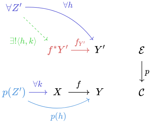
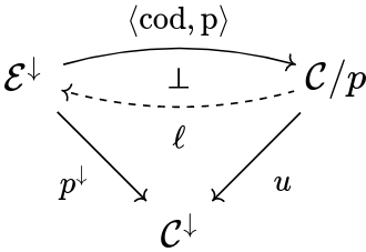
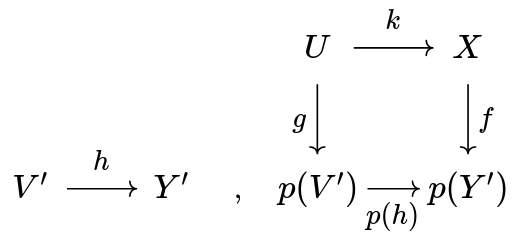
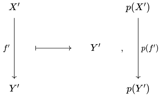
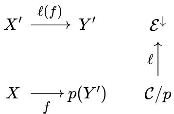
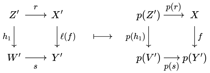
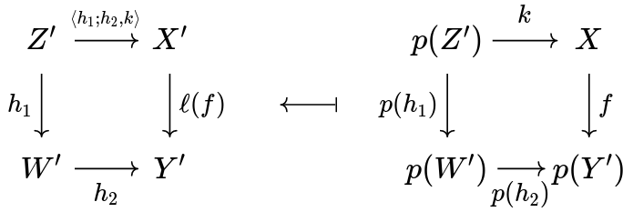
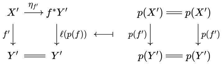
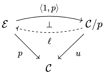
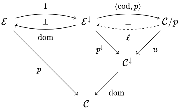
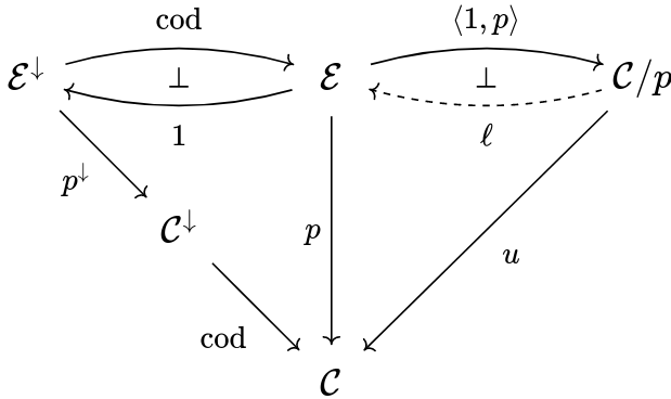

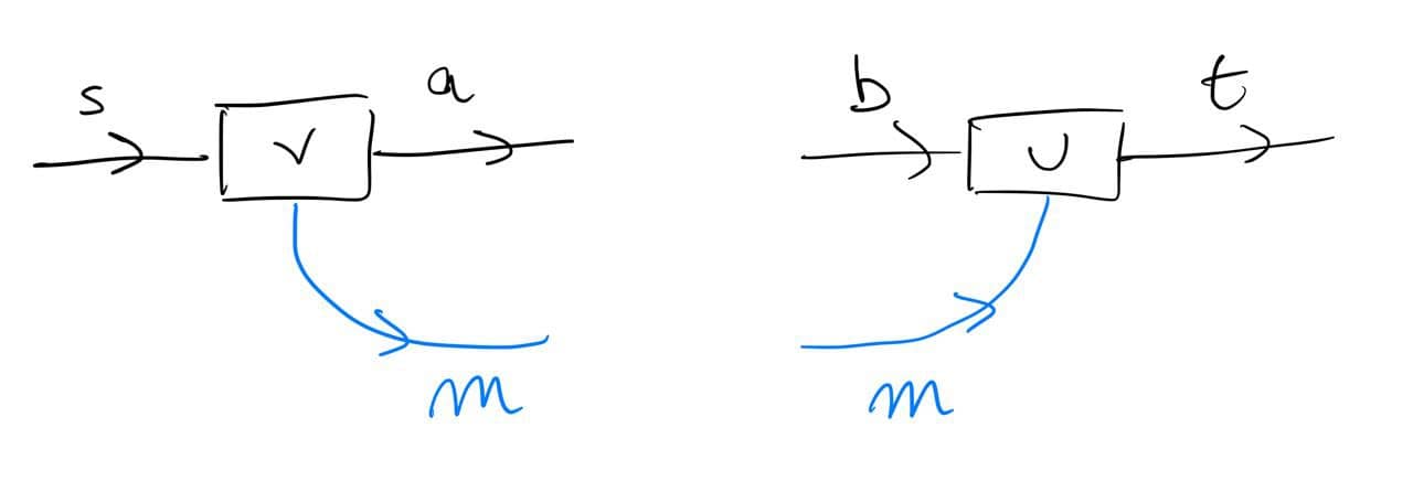
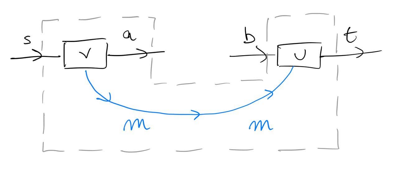
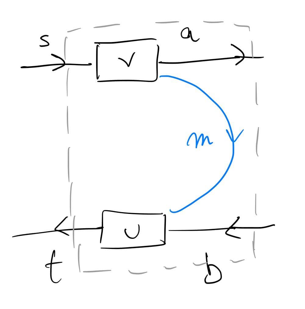
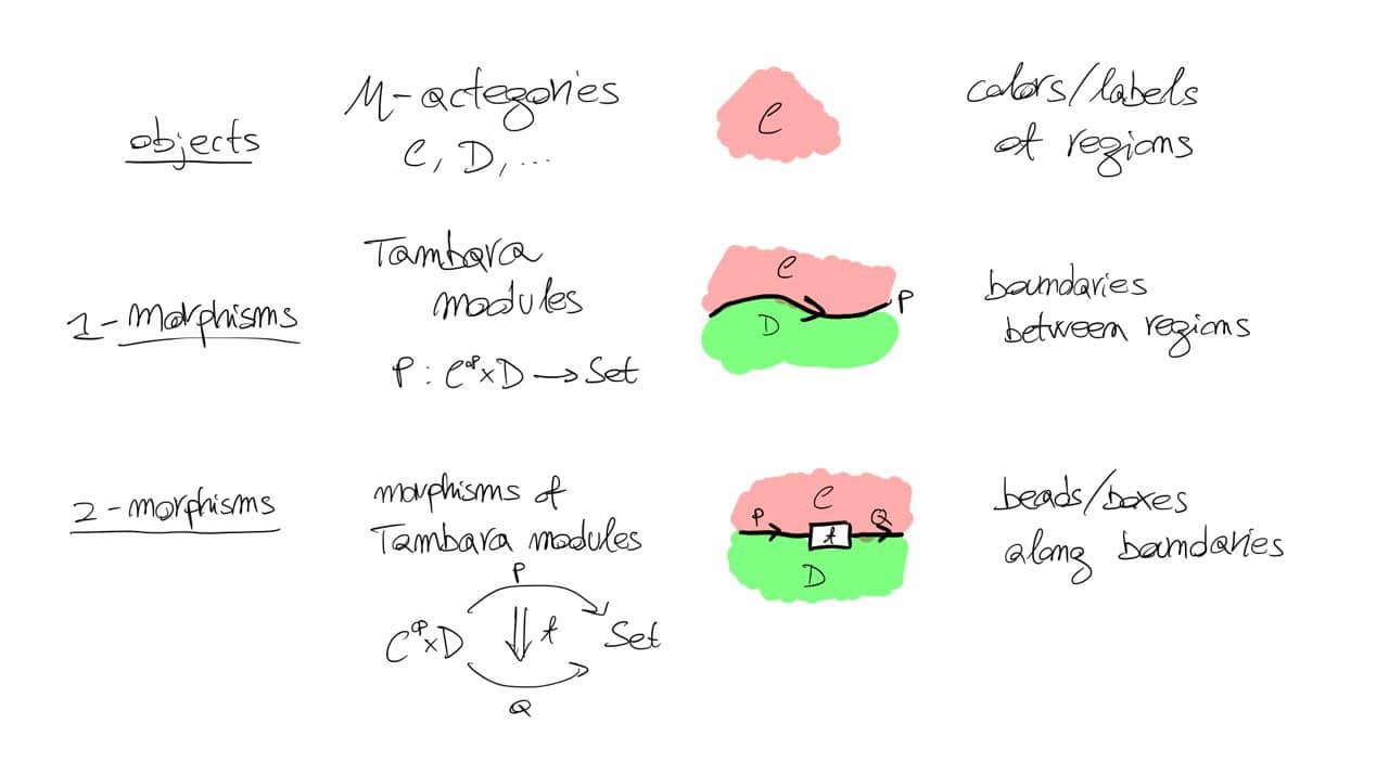
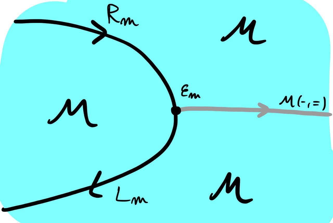
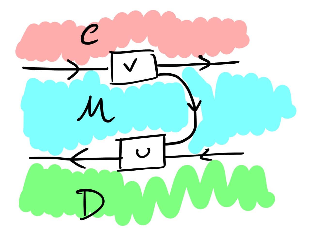
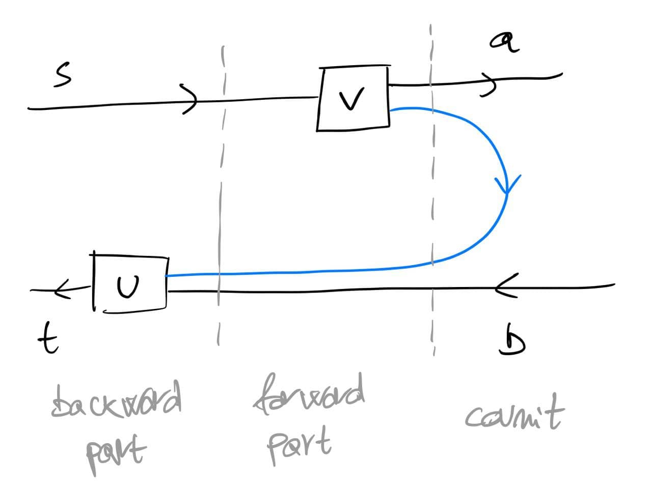
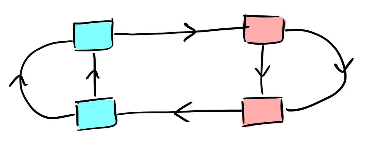
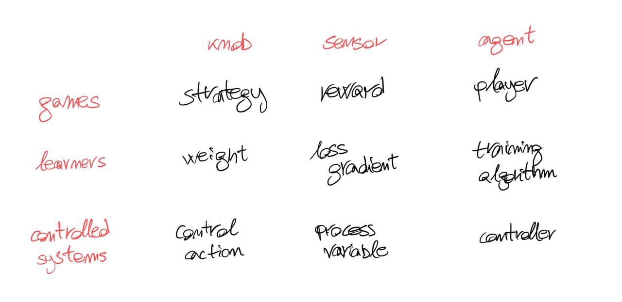

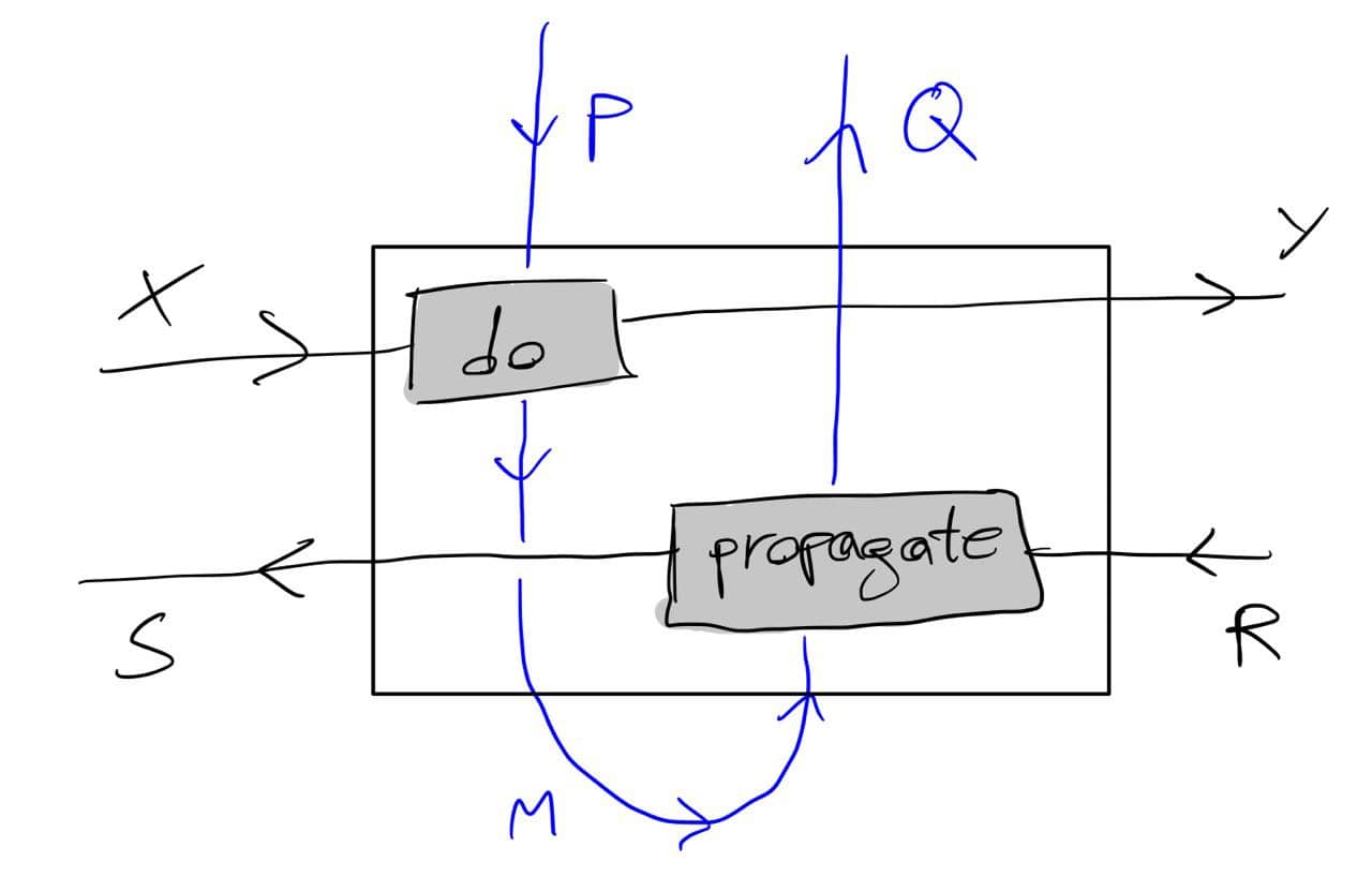
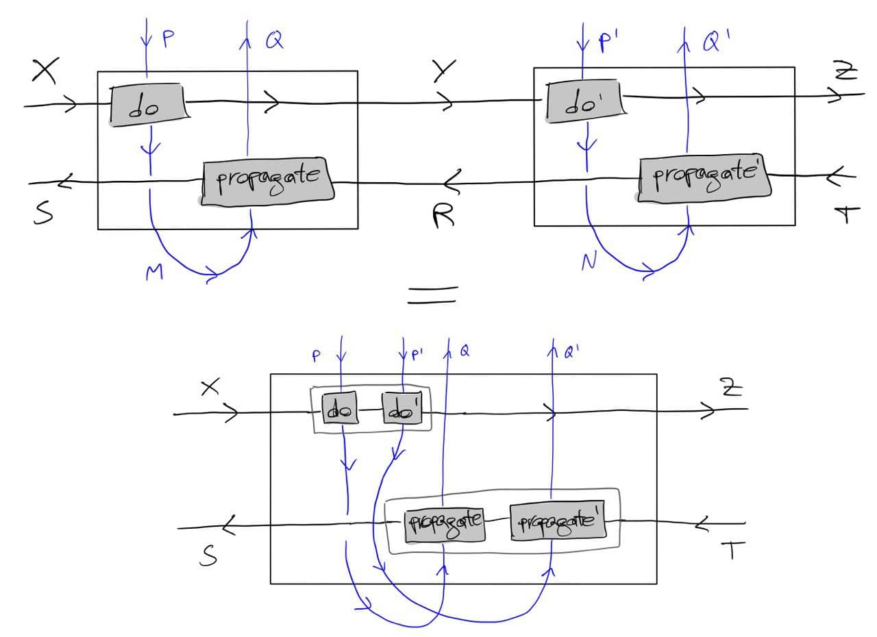
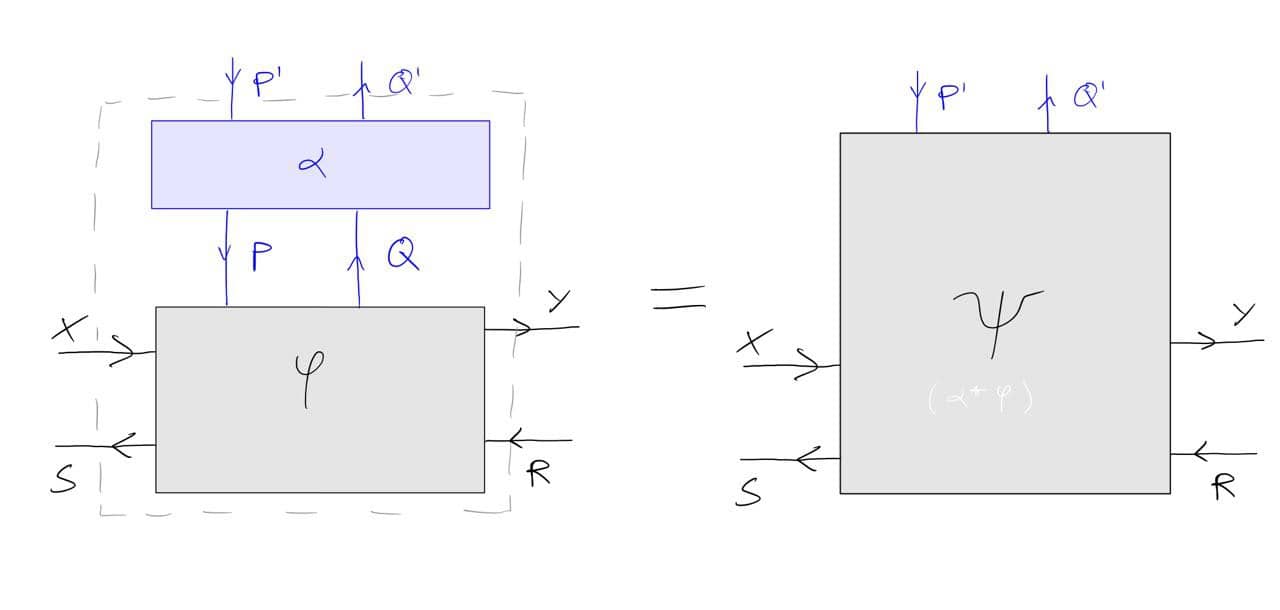
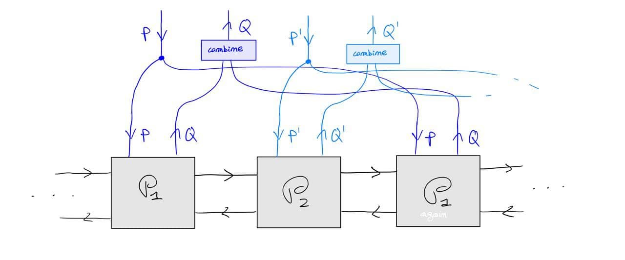
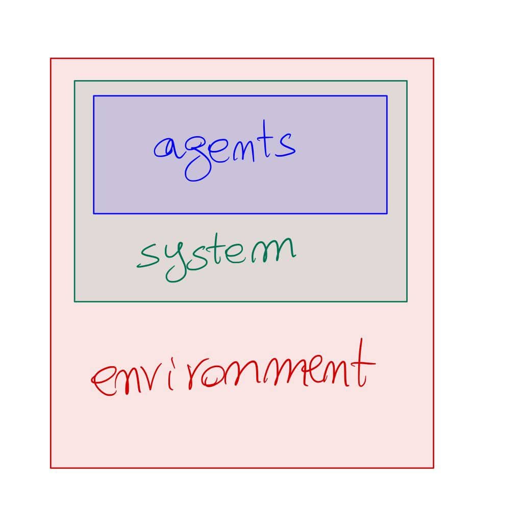
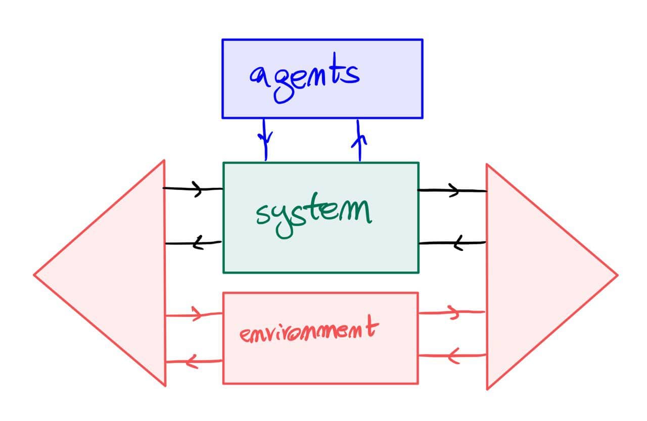
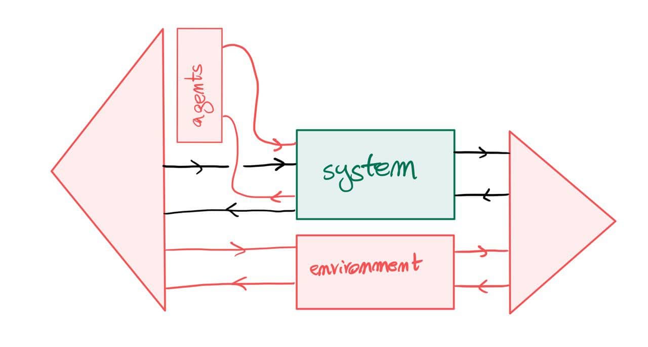
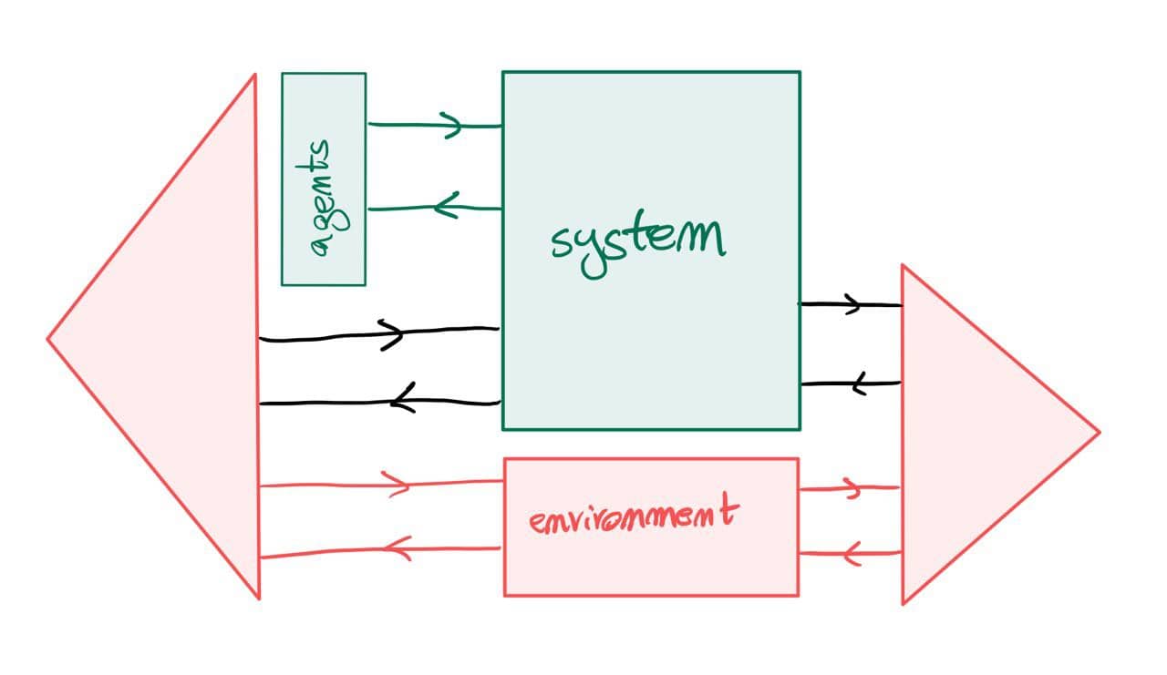
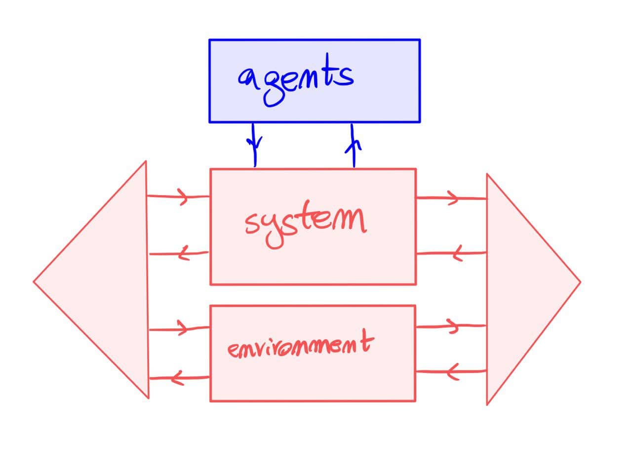
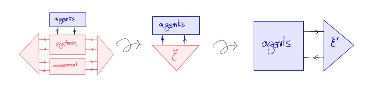
![The dots '...' mean we can repeat the \mathcal G + \mathcal U unit as many times as we want, potentially infinite [7]. The ground symbol is the discard operation, i.e. the unique morphism !_A : A \to 1 from a given set A .](/assets/2021/06/mdp.jpg)
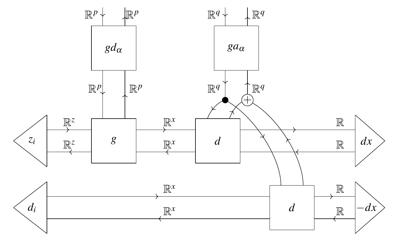
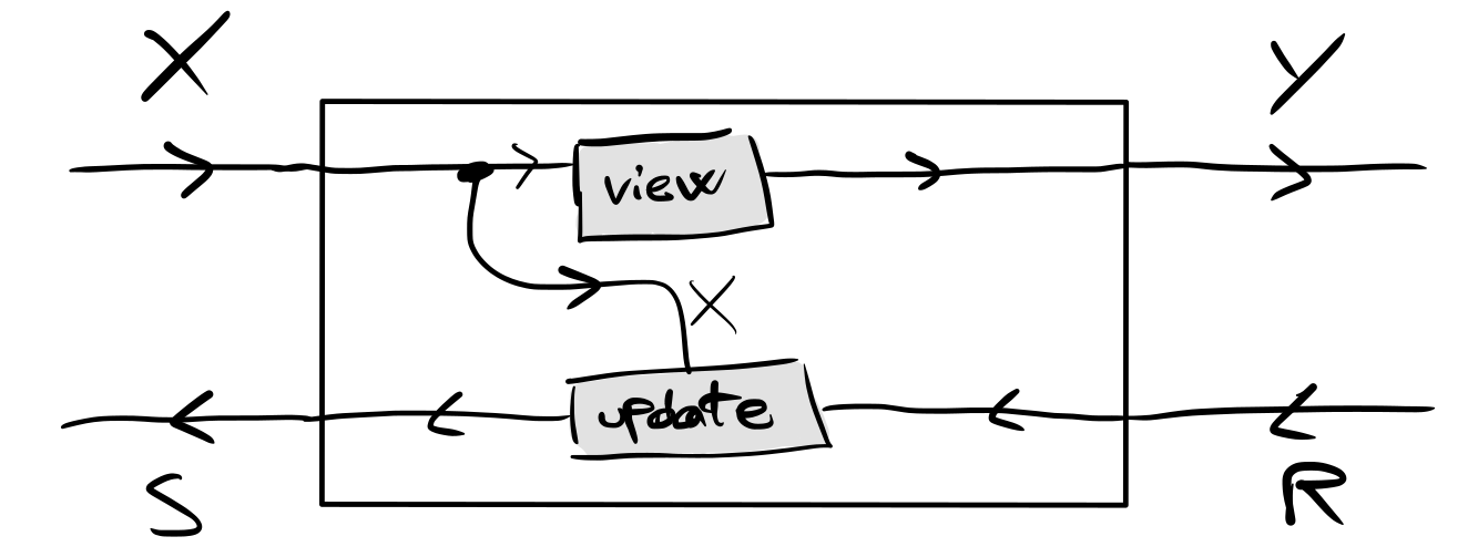
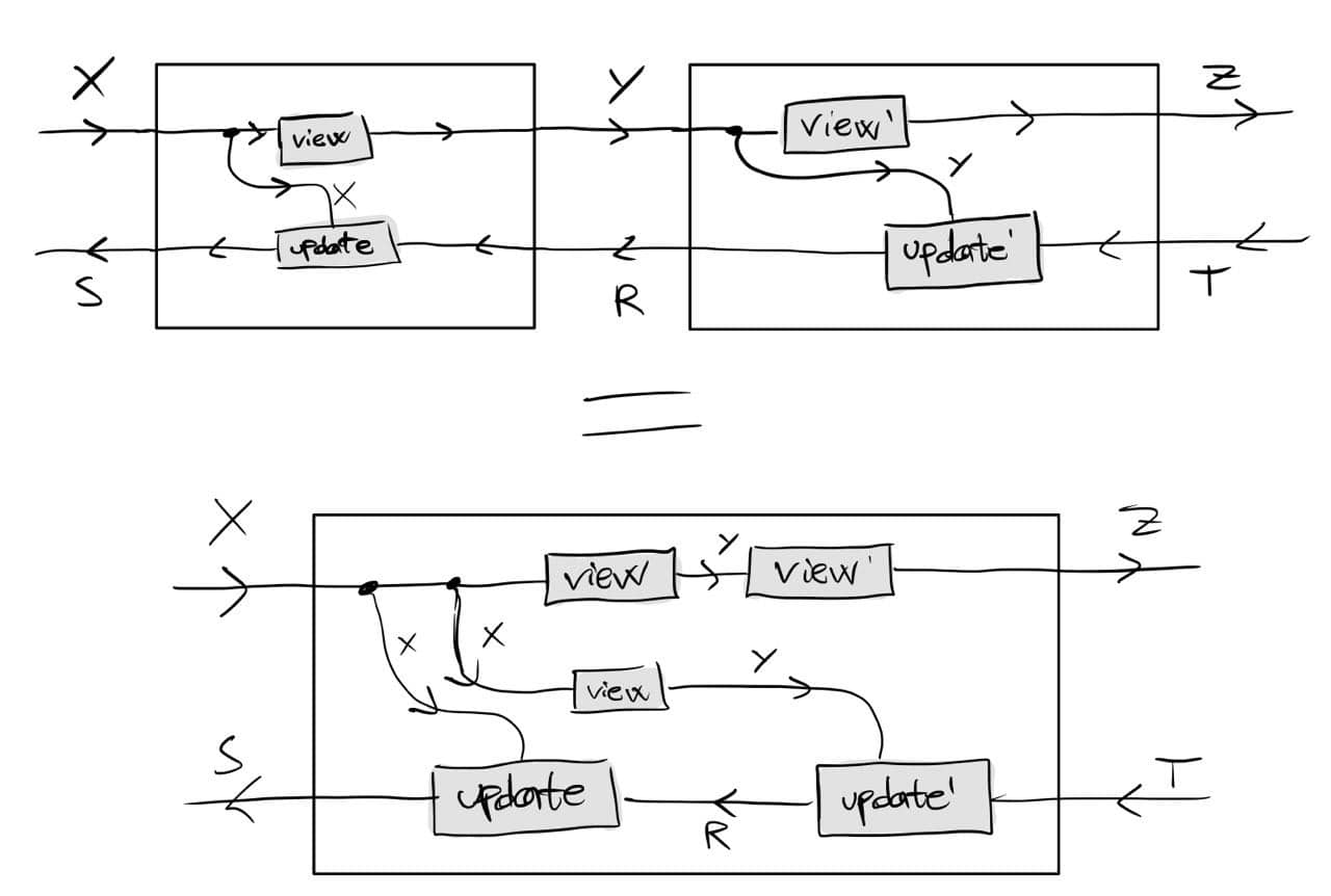
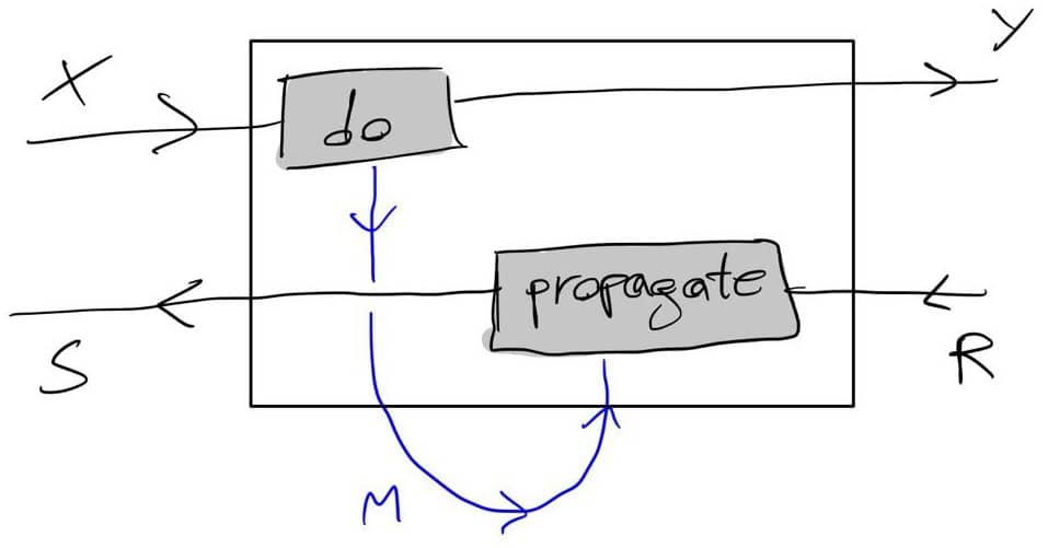
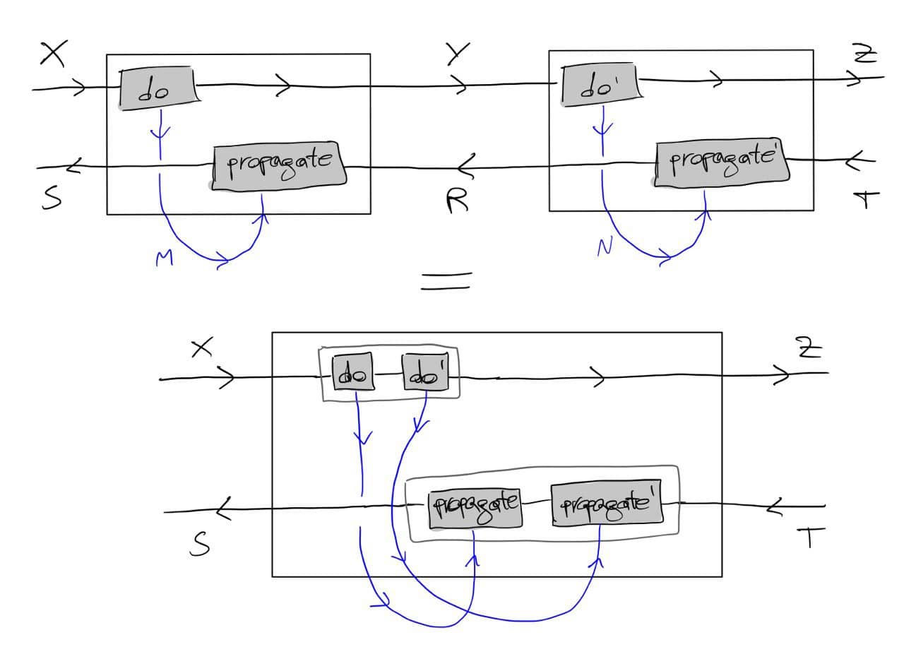
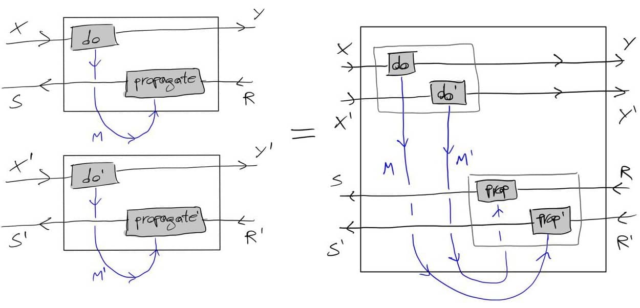
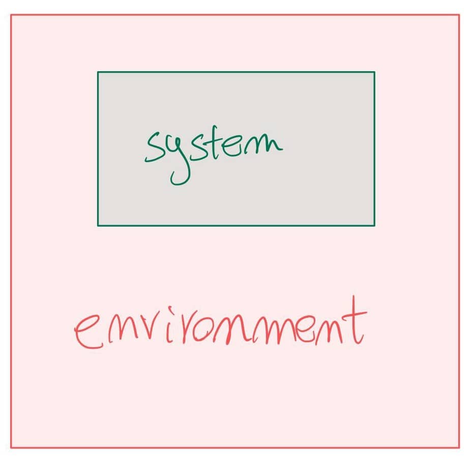
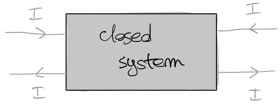
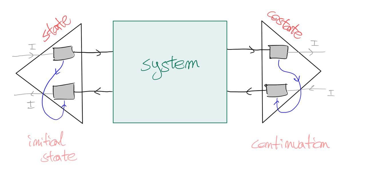
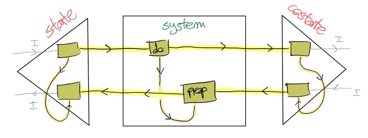
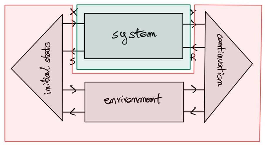
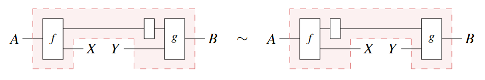
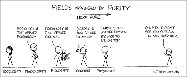